Parametrization
The probability mass function (PMF) for the binomial distribution, considering \(\pmb{y}\) as a vector, is expressed as:
\[f(\pmb{y}) = \prod_{i=1}^{m} \binom{n_i}{y_i} p_i^{y_i} (1 - p_i)^{n_i - y_i},\]
where:
\(\pmb{y} = (y_1, y_2, \ldots, y_m)\) represents a vector of the number of successes for each trial group.
\(\pmb{n} = (n_1, n_2, \ldots, n_m)\) is the vector of the number of trials in each group.
\(\pmb{p} = (p_1, p_2, \ldots, p_m)\) is the vector of probabilities of success in each trial group.
\(y_i = 0, 1, 2, \ldots, n_i\) represents the number of successes in the \(i\)-th trial group.
Assume \(m\) = 1. To demonstrate how different Binomial parameters \(n\) and \(p\) shape the probability mass function (PMF), we create two subplots in Figure 1:
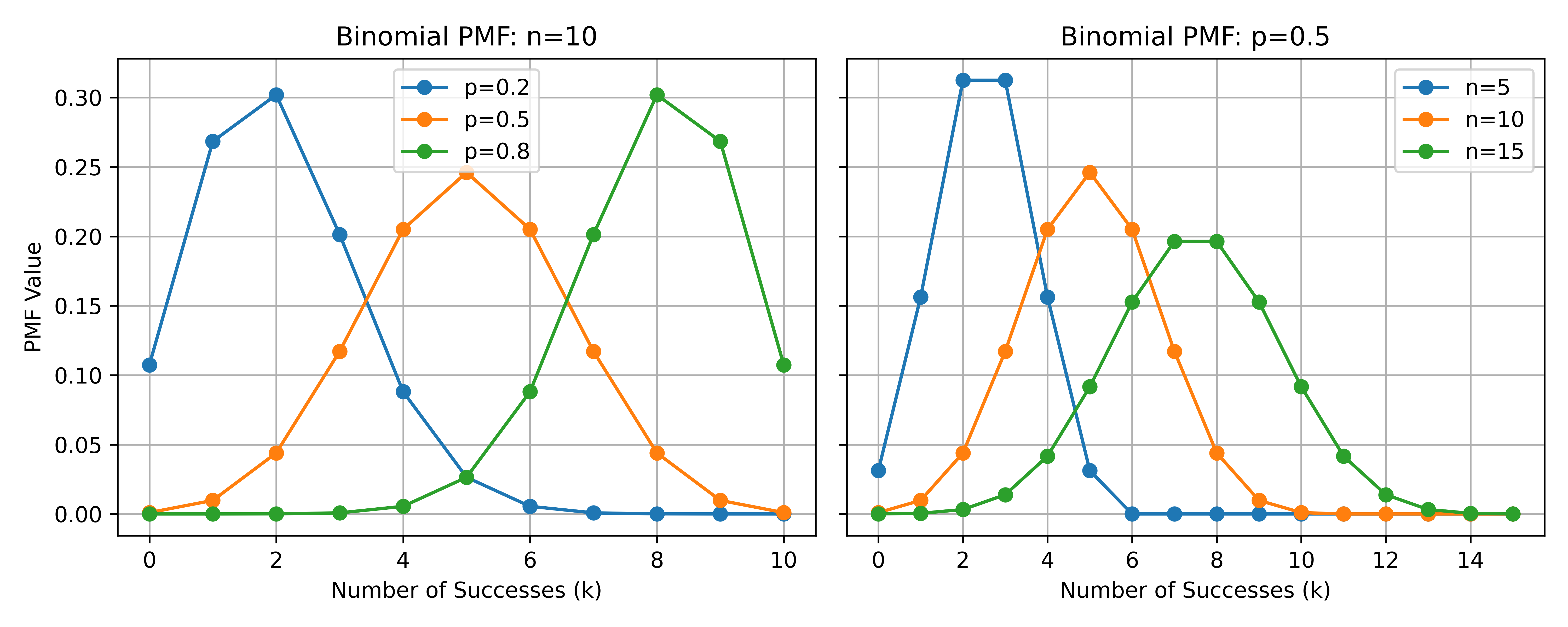
Left plot (fixed \(n=10\)): As \(p\) changes from 0.2 to 0.8, the mass of the distribution shifts from left (fewer successes) to right (more successes).
Right plot (fixed \(p=0.5\)): As \(n\) increases, the possible range of successes expands, resulting in a wider spread of PMF values.
Mean and Variance
The mean and variance vectors for the binomial case are:
\[\pmb{\mu} = \pmb{n} \circ \pmb{p} \quad \text{and} \quad \pmb{\sigma}^2 = \pmb{n} \circ \pmb{p} \circ (1 - \pmb{p}),\]
where \(\circ\) denotes element-wise multiplication.
Link Function
The probability vector \(\pmb{p}\) is linked to the linear predictor vector \(\pmb{\eta}\) via a link function. The default is the logit link:
\[\pmb{p}(\pmb{\eta}) = \frac{\exp(\pmb{\eta})}{1 + \exp(\pmb{\eta})}.\]
Supported link functions:
default: same aslogitlogit(default): \(\eta = \log\bigl(\frac{p}{1-p}\bigr)\)probit: \(\eta = \Phi^{-1}(p)\) where \(\Phi\) is the standard normal CDFcloglog: \(\eta = \log(-\log(1-p))\) (complementary log-log)ccloglog: \(\eta = -\log(-\log(p))\)cauchit: \(\eta = \tan(\pi(p - 0.5))\)log: \(\eta = \log(p)\)loglog: \(\eta = -\log(-\log(p))\)loga: log-a link (requires parameterawith \(0 < a \le 1\) viacontrol={'family': {'link': 'loga', 'control.link': {'a': ...}}})robit: robit link (t-distribution based)sn: skew-normal linkpowerlogit: power logit link
To specify a link function, use control={'family': {'link': 'probit'}}.
Hyperparameters
The binomial likelihood has no hyperparameters. The success probability \(p\) is fully determined by the linear predictor \(\eta\) through the link function.
Validation Rules
pyINLA enforces several validation rules for binomial models to ensure correct specification:
Ntrials Argument
Key: Ntrials
The Ntrials argument specifies the number of trials \(n_i\) for each observation. The validation rules are:
Aggregated binomial: When \(y_i\) can be any integer from 0 to \(n_i\), you must provide
Ntrials.Bernoulli (binary): When all responses are strictly 0 or 1,
Ntrialscan be omitted (implicitly \(n_i = 1\)).Length requirement:
Ntrialsmust have the same length as the response vector.Positive integers: All entries in
Ntrialsmust be positive integers.
# Bernoulli (binary 0/1): Ntrials not required
result = pyinla(model={'response': 'y', 'fixed': ['1', 'x']}, family="binomial", data=df)

# Aggregated binomial: Ntrials required
result = pyinla(model={'response': 'successes', 'fixed': ['1', 'x']}, family="binomial", data=df, Ntrials=df["trials"])
Link Function
Key: control['family']['link']
The link function can be specified via the control dictionary. If not specified, the default logit link is used.
# Default logit link
result = pyinla(model={'response': 'y', 'fixed': ['1', 'x']}, family="binomial", data=df)

# Probit link
result = pyinla(model={'response': 'y', 'fixed': ['1', 'x']}, family="binomial", data=df,
                control={'family': {'link': 'probit'}})

# Complementary log-log link
result = pyinla(model={'response': 'y', 'fixed': ['1', 'x']}, family="binomial", data=df,
                control={'family': {'link': 'cloglog'}})
Variant Parameter
Key: control['family']['variant']
The variant parameter selects between the standard binomial and the negative binomial variant:
variant=0(default): Standard binomial distribution.variant=1: Negative binomial variant (see section below).
# Standard binomial (default).
# Here `y` is the per-row success count (0..n), and `Ntrials` is the trial
# count per row. variant=1 only converges on aggregated counts; do NOT pass
# a Bernoulli (0/1) `y` here (use the no-`Ntrials` form from the chunk above
# for binary data).
Ntrials = df["n"].to_numpy()
result = pyinla(model={'response': 'y', 'fixed': ['1', 'x']}, family="binomial", data=df, Ntrials=Ntrials)

# Negative binomial variant (requires aggregated `y`)
result = pyinla(model={'response': 'y', 'fixed': ['1', 'x']}, family="binomial", data=df, Ntrials=Ntrials,
                control={'family': {'variant': 1}})
Response Values
Response variable \(\pmb{y}\) must satisfy:
All values must be non-negative integers (0, 1, 2, ...)
All values must be less than or equal to the corresponding
Ntrialsvalue
pyINLA will raise PyINLAError if any response value is negative, non-integer, or exceeds its trial count.
Specification
family="binomial"Required arguments:
\(\pmb y\) and \(\pmb n\): observed data (\(y_i\) for each observation) and trials (
Ntrials).
Optional arguments:
control={'family': {'variant': 0}}for standard binomial (default), andcontrol={'family': {'variant': 1}}for the negative binomial variant.
Negative Binomial Variant
When variant=1 is specified, the negative binomial distribution is used instead of the standard binomial. The probability mass function is:
\[f(\pmb{n}) = \prod_{i=1}^{m} \binom{n_i-1}{y_i-1} p_i^{y_i} (1-p_i)^{n_i-y_i}\]
for given \(\pmb{y} = (y_1, y_2, \ldots, y_m)\) where \(y_i = 1, 2, \ldots\), and response \(n_i - y_i = 0, 1, 2, \ldots\).
Note: In this variant, the "data" enters via the Ntrials argument (since \(\pmb{y}\) is predetermined), which may seem unconventional.
Specification for Expert Version
family="xbinomial"Required arguments:
\(\pmb y\) and \(\pmb n\): observed data (\(y_i\) for each observation) and trials (
Ntrials).
Optional arguments:
scale=q, which scales the probability with \(0< \pmb q \le1\) into \(\pmb p'\), where \[\pmb p' = \pmb q \pmb p( \pmb \eta).\] By default, \(\pmb q= \pmb 1\). Note that “fitted values” will still be be \(\pmb p(\pmb \eta)\).
Expert version notes: The expert version (xbinomial) allows non-integer values for both \(\pmb{y}\) and \(\pmb{n}\). The condition \(0 \le y_i \le n_i\) still applies. The normalizing constant is computed using the integer parts (floor) of \(y\) and \(n\). Note that this extension can make the marginal likelihood estimate less interpretable.
Note: If the response is a factor, it must be converted to {0, 1} before calling pyinla(), as this conversion is not done automatically.