Negative Binomial Variant

Introduction

In this tutorial, we demonstrate how to use the binomial family with the variant=1 option to fit a negative binomial model. This variant is useful when modeling the number of failures before a given number of successes is achieved.

The negative binomial variant swaps the roles of successes and failures, with the "data" entering through the Ntrials argument rather than the response.

The Model

When variant=1 is specified, the negative binomial distribution is used instead of the standard binomial. The probability mass function is:

f(\pmb{n}) = \prod_{i=1}^{m} \binom{n_i-1}{y_i-1} p_i^{y_i} (1-p_i)^{n_i-y_i}

where:

$\pmb{y} = (y_1, y_2, \ldots, y_m)$ is the vector of predetermined number of successes (fixed values)
$\pmb{n} = (n_1, n_2, \ldots, n_m)$ is the response: $n_i - y_i$ represents the number of failures
$\pmb{p} = (p_1, p_2, \ldots, p_m)$ is the vector of success probabilities
$y_i = 1, 2, \ldots$ and $n_i - y_i = 0, 1, 2, \ldots$

Note: In this variant, the "data" enters via the Ntrials argument (since $\pmb{y}$ is predetermined), which may seem unconventional.

Linear Predictor

The linear predictor $\eta_i$ links the log-odds of success to the covariates:

\eta_i = \beta_0 + \beta_1 z_i

where $\beta_0$ is the intercept and $\beta_1$ is the slope coefficient for covariate $z_i$.

The probability of success is:

p_i = \frac{\exp(\eta_i)}{1 + \exp(\eta_i)} = \text{logit}^{-1}(\eta_i)

Hyperparameters

Like the standard binomial, the negative binomial variant has no hyperparameters. The model is fully determined by the regression coefficients $\boldsymbol{\beta}$.

Dataset

The dataset contains $n = 100$ observations with three columns:

Column	Description	Type
`y`	Number of successes (predetermined)	integer
`z`	Covariate (predictor variable)	float
`Ntrials`	Total count ($y + \text{failures}$)	integer

dataset_nbinomial.csv

Download the CSV file and place it in your working directory.

Implementation in pyINLA

We fit the model using pyINLA by specifying control_family={'variant': 1}:

Load the data into a pandas DataFrame
Extract the Ntrials vector
Define the model structure (response and fixed effects)
Call pyinla() with family='binomial' and control_family={'variant': 1}

import pandas as pd
from pyinla import pyinla

# Load data
df = pd.read_csv('dataset_nbinomial.csv')
Ntrials = df['Ntrials'].to_numpy()

# Define model: y ~ 1 + z (intercept + slope)
model = {
    'response': 'y',
    'fixed': ['1', 'z']
}

# Fit the negative binomial variant model
result = pyinla(
    model=model,
    family='binomial',
    data=df,
    Ntrials=Ntrials,
    control_family={'variant': 1}
)

# View posterior summaries for fixed effects
print(result.summary_fixed)

Extracting Results

The result object contains all posterior inference:

# Fixed effects: posterior summaries for beta_0 and beta_1
print(result.summary_fixed)

# Extract posterior means
intercept = result.summary_fixed.loc['(Intercept)', 'mean']
slope = result.summary_fixed.loc['z', 'mean']

# Compute predicted probabilities
import numpy as np
eta_hat = intercept + slope * df['z'].to_numpy()
p_hat = np.exp(eta_hat) / (1 + np.exp(eta_hat))

The summary_fixed DataFrame includes columns for mean, sd, 0.025quant, 0.5quant, 0.975quant, and mode.

Results and Diagnostics

The posterior summaries provide point estimates and credible intervals for $\beta_0$ and $\beta_1$.

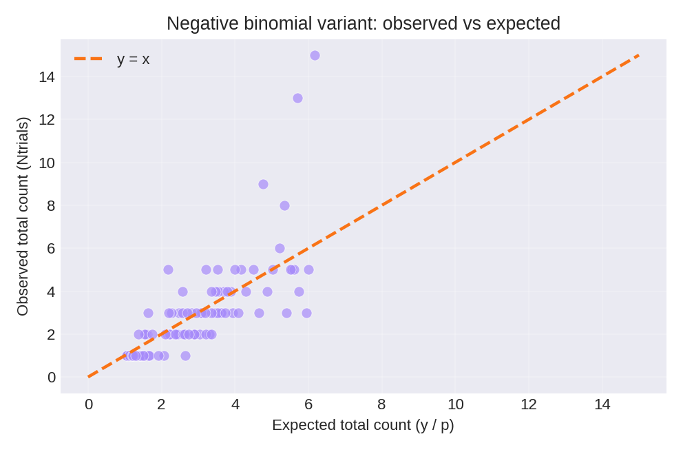
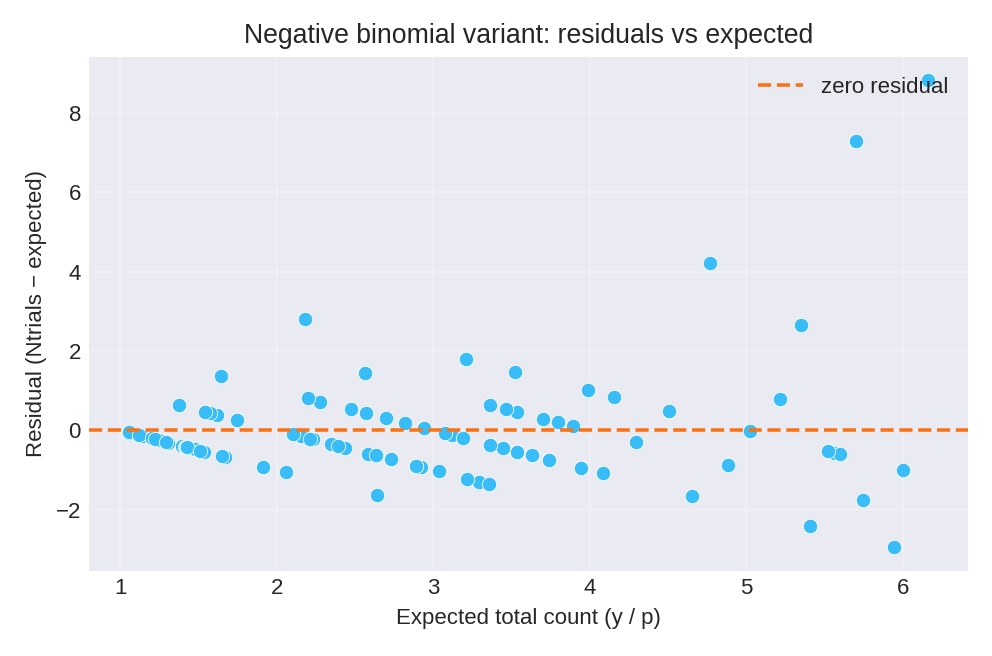
Observed Ntrials vs expected total count — Observed total count (Ntrials) versus expected total count $y_i / \hat{p}_i$.

Residuals versus expected total count — Residuals (Ntrials $- y_i / \hat{p}_i$) versus expected total count.

To reproduce these figures locally, download the render_nbinomial_plots.py script and run it alongside the CSV dataset.

Data Generation (Reference)

For reproducibility, the dataset was simulated from the following data-generating process:

z_i \stackrel{\text{iid}}{\sim} \mathcal{N}(0, 1), \quad y_i \sim \text{Uniform}\{1, 2, 3\}, \quad n_i = y_i + \text{NegBin}(y_i, p_i)

where $p_i = \text{logit}^{-1}(\beta_0 + \beta_1 z_i)$ with true parameter values: $\beta_0 = 1$, $\beta_1 = 1$.

# Data generation script (for reference only)
import numpy as np
import pandas as pd

rng = np.random.default_rng(2026)
n = 100
beta0, beta1 = 1.0, 1.0

z = rng.normal(size=n)
eta = beta0 + beta1 * z
prob = np.exp(eta) / (1 + np.exp(eta))

# y is predetermined number of successes
y = rng.integers(1, 4, size=n)  # y = sample(1:3, size=n, replace=TRUE)
# Ntrials = y + number of failures (negative binomial)
Ntrials = y + rng.negative_binomial(n=y, p=prob)

df = pd.DataFrame({'y': y, 'z': np.round(z, 6), 'Ntrials': Ntrials})
# df.to_csv('dataset_nbinomial.csv', index=False)