Binomial Regression

Introduction

In this tutorial, we fit a Bayesian binomial regression model for binary outcome data. The binomial distribution is the natural choice for modeling the number of successes in a fixed number of independent trials, each with the same probability of success.

Binomial regression is widely used in epidemiology, clinical trials, and social sciences where outcomes are counts of successes out of a known number of trials.

The Model

We consider a binomial regression model with $n$ observations. For each observation $i = 1, \ldots, n$, the count of successes $y_i$ out of $N_i$ trials is modeled as:

y_i \sim \text{Binomial}(N_i, p_i)

where:

$y_i \in \{0, 1, 2, \ldots, N_i\}$ is the observed number of successes
$N_i > 0$ is the known number of trials for observation $i$
$p_i \in (0, 1)$ is the probability of success

The probability mass function is:

P(y_i \mid N_i, p_i) = \binom{N_i}{y_i} p_i^{y_i} (1 - p_i)^{N_i - y_i}

Linear Predictor

The linear predictor $\eta_i$ links the log-odds of success to the covariates through a linear combination:

\eta_i = \beta_0 + \beta_1 z_i

where $\beta_0$ is the intercept and $\beta_1$ is the slope coefficient for covariate $z_i$.

The binomial distribution uses the logit link function, so the probability of success is:

p_i = \frac{\exp(\eta_i)}{1 + \exp(\eta_i)} = \text{logit}^{-1}(\eta_i)

Equivalently:

\text{logit}(p_i) = \log\left(\frac{p_i}{1 - p_i}\right) = \eta_i

Likelihood Function

The likelihood for the full dataset $\mathbf{y} = (y_1, \ldots, y_n)^\top$ is:

p(\mathbf{y} \mid \boldsymbol{\beta}, \mathbf{N}) = \prod_{i=1}^{n} \binom{N_i}{y_i} p_i^{y_i} (1 - p_i)^{N_i - y_i}

where $p_i = \text{logit}^{-1}(\beta_0 + \beta_1 z_i)$ and $\boldsymbol{\beta} = (\beta_0, \beta_1)^\top$.

Hyperparameters

The binomial likelihood has no hyperparameters. The variance is determined by the mean:

\text{Var}(y_i) = N_i \cdot p_i \cdot (1 - p_i)

This means there are no additional variance parameters to estimate. The model is fully determined by the regression coefficients $\boldsymbol{\beta}$.

Dataset

The dataset contains $n = 100$ observations with three columns:

Column	Description	Type
`y`	Number of successes	integer
`z`	Covariate (predictor variable)	float
`Ntrials`	Number of trials	integer

dataset_binomial_regression.csv

Download the CSV file and place it in your working directory.

Implementation in pyINLA

We fit the model using pyINLA. The key steps are:

Load the data into a pandas DataFrame
Extract the Ntrials vector
Define the model structure (response and fixed effects)
Call pyinla() with family='binomial' and the Ntrials vector

import pandas as pd
from pyinla import pyinla

# Load data
df = pd.read_csv('dataset_binomial_regression.csv')
Ntrials = df['Ntrials'].to_numpy()

# Define model: y ~ 1 + z (intercept + slope)
model = {
    'response': 'y',
    'fixed': ['1', 'z']
}

# Fit the binomial regression model
result = pyinla(
    model=model,
    family='binomial',
    data=df,
    Ntrials=Ntrials
)

# View posterior summaries for fixed effects
print(result.summary_fixed)

Extracting Results

The result object contains all posterior inference:

# Fixed effects: posterior summaries for beta_0 and beta_1
print(result.summary_fixed)

# Extract posterior means
intercept = result.summary_fixed.loc['(Intercept)', 'mean']
slope = result.summary_fixed.loc['z', 'mean']

# Compute predicted probabilities
import numpy as np
eta_hat = intercept + slope * df['z'].to_numpy()
p_hat = np.exp(eta_hat) / (1 + np.exp(eta_hat))

# Compute expected counts
expected_counts = df['Ntrials'].to_numpy() * p_hat

The summary_fixed DataFrame includes columns for mean, sd, 0.025quant, 0.5quant, 0.975quant, and mode.

Results and Diagnostics

The posterior summaries provide point estimates and credible intervals for $\beta_0$ and $\beta_1$.

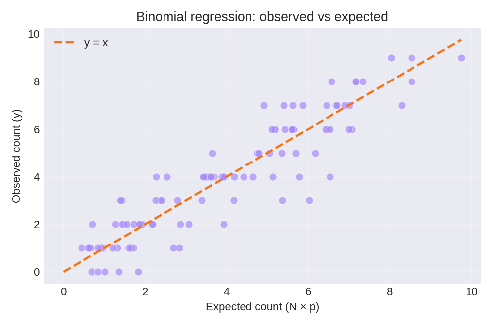
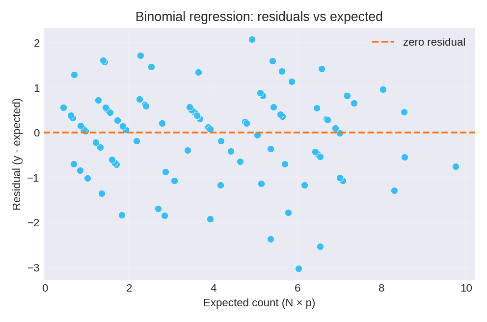
Observed vs expected counts — Observed counts $y_i$ versus expected counts $N_i \hat{p}_i$. Points near the diagonal indicate good fit.

Residuals versus expected counts — Residuals $y_i - N_i \hat{p}_i$ versus expected counts.

To reproduce these figures locally, download the render_binomial_plots.py script and run it alongside the CSV dataset.

Data Generation (Reference)

For reproducibility, the dataset was simulated from the following data-generating process:

z_i \stackrel{\text{iid}}{\sim} \mathcal{N}(0, 1), \quad N_i \sim \text{Uniform}\{1, 2, \ldots, 10\}, \quad y_i \sim \text{Binomial}(N_i, p_i)

where $p_i = \text{logit}^{-1}(\beta_0 + \beta_1 z_i)$ with true parameter values: $\beta_0 = 1$, $\beta_1 = 1$.

# Data generation script (for reference only)
import numpy as np
import pandas as pd

rng = np.random.default_rng(2026)
n = 100
beta0, beta1 = 1.0, 1.0

z = rng.normal(size=n)
Ntrials = rng.integers(1, 11, size=n)  # trials between 1 and 10
eta = beta0 + beta1 * z
p = np.exp(eta) / (1 + np.exp(eta))
y = rng.binomial(n=Ntrials, p=p)

df = pd.DataFrame({'y': y, 'z': np.round(z, 6), 'Ntrials': Ntrials})
# df.to_csv('dataset_binomial_regression.csv', index=False)