Expert Binomial with Scale

Introduction

In this tutorial, we demonstrate the expert version of the binomial distribution (xbinomial) with a scale parameter. This is useful when the success probability needs to be scaled by a known factor for each observation.

The expert version also allows non-integer values for both $\pmb{y}$ and $\pmb{n}$, providing more flexibility for specialized modeling scenarios.

The Model

We consider an expert binomial regression model with $n$ observations. For each observation $i = 1, \ldots, n$, the count of successes $y_i$ out of $N_i$ trials is modeled as:

y_i \sim \text{Binomial}(N_i, p'_i)

where the effective probability $p'_i$ is scaled:

p'_i = q_i \cdot p_i(\eta_i)

and:

$y_i \in \{0, 1, 2, \ldots, N_i\}$ is the observed number of successes
$N_i > 0$ is the known number of trials for observation $i$
$q_i \in (0, 1]$ is the known scale factor for observation $i$
$p_i(\eta_i) = \text{logit}^{-1}(\eta_i)$ is the base probability from the linear predictor

Note: The "fitted values" reported by pyINLA will be $p(\eta)$, not $p' = q \cdot p(\eta)$.

Linear Predictor

The linear predictor $\eta_i$ links the log-odds of the base probability to the covariates:

\eta_i = \beta_0 + \beta_1 x_i

where $\beta_0$ is the intercept and $\beta_1$ is the slope coefficient for covariate $x_i$.

The base probability is:

p_i = \frac{1}{1 + \exp(-\eta_i)}

And the effective probability used in the binomial likelihood is:

p'_i = q_i \cdot p_i

Hyperparameters

Like the standard binomial, the expert binomial has no hyperparameters. The variance is determined by the mean:

\text{Var}(y_i) = N_i \cdot p'_i \cdot (1 - p'_i)

Dataset

The dataset contains $n = 10,000$ observations with four columns:

Column	Description	Type
`y`	Number of successes	integer
`x`	Covariate (predictor variable)	float
`q`	Scale factor ($0 < q \le 1$)	float
`ntrials`	Number of trials	integer

dataset_xbinomial.csv

Download the CSV file and place it in your working directory.

Implementation in pyINLA

We fit the model using pyINLA with family='xbinomial' and the scale parameter:

Load the data into a pandas DataFrame
Extract the ntrials and scale (q) vectors
Define the model structure (response and fixed effects)
Call pyinla() with family='xbinomial', Ntrials, and scale

import pandas as pd
from pyinla import pyinla

# Load data
df = pd.read_csv('dataset_xbinomial.csv')
ntrials = df['ntrials'].to_numpy()
q = df['q'].to_numpy()

# Define model: y ~ 1 + x (intercept + slope)
model = {
    'response': 'y',
    'fixed': ['1', 'x']
}

# Fit the expert binomial model with scale
result = pyinla(
    model=model,
    family='xbinomial',
    data=df,
    Ntrials=ntrials,
    scale=q
)

# View posterior summaries for fixed effects
print(result.summary_fixed)

Extracting Results

The result object contains all posterior inference:

# Fixed effects: posterior summaries for beta_0 and beta_1
print(result.summary_fixed)

# Extract posterior means
intercept = result.summary_fixed.loc['(Intercept)', 'mean']
slope = result.summary_fixed.loc['x', 'mean']

# Compute predicted base probabilities (not scaled)
import numpy as np
eta_hat = intercept + slope * df['x'].to_numpy()
p_hat = 1.0 / (1 + np.exp(-eta_hat))

# Compute effective probabilities (with scale)
p_effective = df['q'].to_numpy() * p_hat

# Compute expected counts
expected_counts = df['ntrials'].to_numpy() * p_effective

The summary_fixed DataFrame includes columns for mean, sd, 0.025quant, 0.5quant, 0.975quant, and mode.

Results and Diagnostics

The posterior summaries provide estimates for $\beta_0$ and $\beta_1$. The true parameters used for data generation were $\beta_0 = 0.88$ and $\beta_1 = 0.77$.

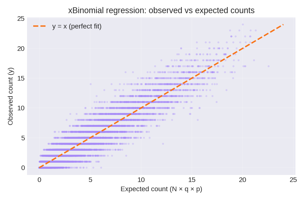
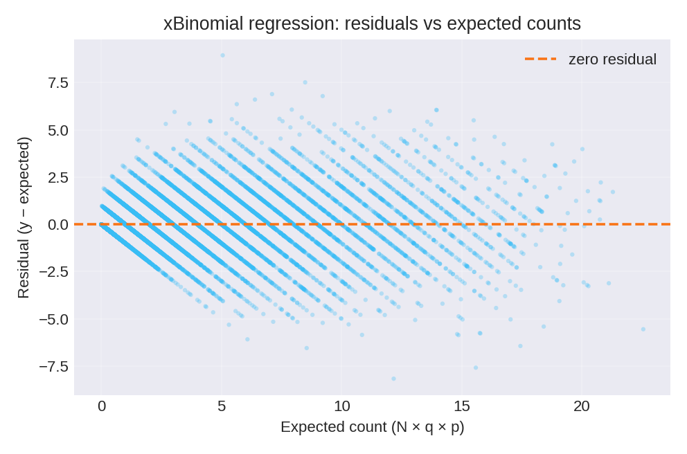
Scatter plot of observed vs expected counts with perfect-fit line — Observed counts $y_i$ versus expected counts $N_i \cdot q_i \cdot \hat{p}_i$.

Residuals versus expected counts — Residuals $y_i - N_i q_i \hat{p}_i$ versus expected counts.

To reproduce these figures locally, download the render_xbinomial_plots.py script and run it alongside the CSV dataset.

Data Generation (Reference)

For reproducibility, the dataset was simulated from the following data-generating process:

x_i \stackrel{\text{iid}}{\sim} \mathcal{N}(0, 1), \quad q_i \sim \text{Uniform}(0, 1), \quad N_i \sim \text{Uniform}\{1, 2, \ldots, 25\}

p'_i = q_i \cdot \frac{1}{1 + \exp(-\eta_i)}, \quad y_i \sim \text{Binomial}(N_i, p'_i)

where $\eta_i = \beta_0 + \beta_1 x_i$ with true parameter values: $\beta_0 = 0.88$, $\beta_1 = 0.77$.

# Data generation script (for reference only)
import numpy as np
import pandas as pd

rng = np.random.default_rng(123)
n = 10000
beta0, beta1 = 0.88, 0.77

x = rng.normal(size=n)
q = rng.uniform(0, 1, size=n)  # scale factors
eta = beta0 + beta1 * x
p = 1.0 / (1 + np.exp(-eta))
p_scaled = q * p
ntrials = rng.integers(1, 26, size=n)  # trials between 1 and 25
y = rng.binomial(n=ntrials, p=p_scaled)

df = pd.DataFrame({
    'y': y,
    'x': np.round(x, 6),
    'q': np.round(q, 6),
    'ntrials': ntrials
})
# df.to_csv('dataset_xbinomial.csv', index=False)