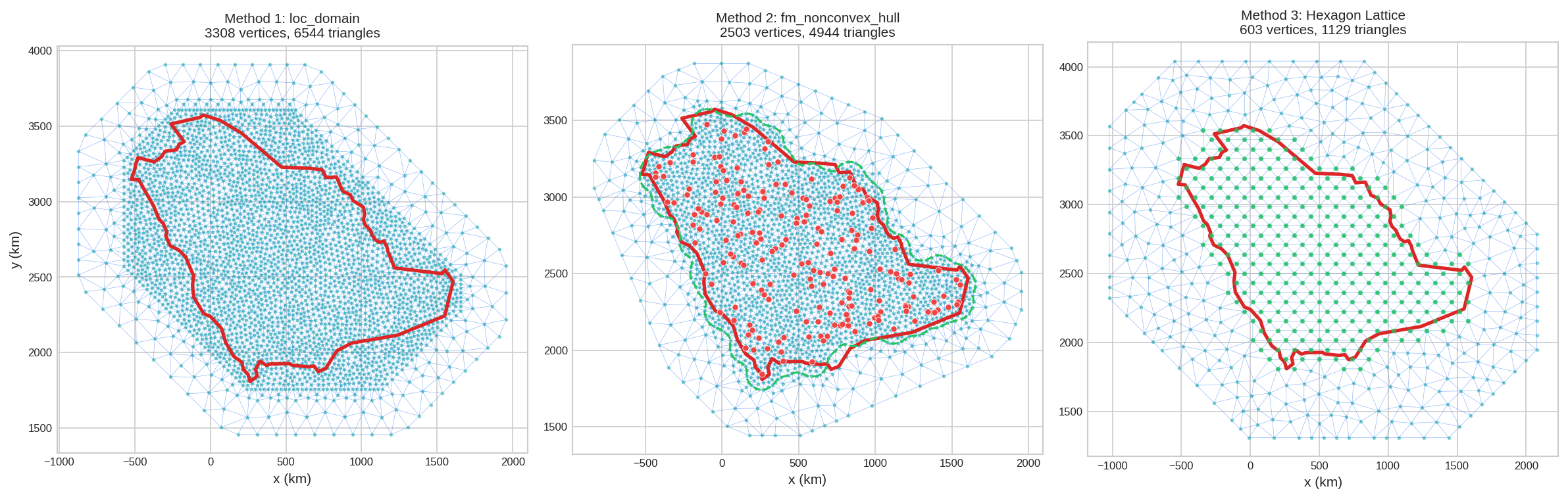
Overview: Three Approaches
When working with geographic regions (countries, study areas), there are three main ways to create a mesh:
| Method | Input Required | When to Use | Pros |
|---|---|---|---|
| 1. loc_domain | Boundary polygon only | You have the exact study area boundary | Uses exact boundary shape |
| 2. fm_nonconvex_hull | Data/observation points | You have scattered data points | Adapts to point distribution |
| 3. fm_hexagon_lattice | Boundary polygon only | Uniform prediction grid needed | Uniform vertex spacing |
Setup: Loading a Country Boundary
We'll use Saudi Arabia as an example. First, load the boundary and project to a suitable CRS (in kilometers):
import numpy as np
import geopandas as gpd
from shapely.geometry import Polygon
from pyinla.fmesher import fm_mesh_2d, fm_nonconvex_hull, fm_hexagon_lattice

# Load Saudi Arabia boundary from Natural Earth
url = 'https://naciscdn.org/naturalearth/110m/cultural/ne_110m_admin_0_countries.zip'
world = gpd.read_file(url)
saudi = world[world['ADMIN'] == 'Saudi Arabia']

# Project to UTM zone 38N directly in kilometers
saudi_km = saudi.to_crs("+proj=utm +zone=38 +units=km")

# Get bounding box
bounds = saudi_km.total_bounds  # [minx, miny, maxx, maxy]
width = bounds[2] - bounds[0]
height = bounds[3] - bounds[1]
print(f"Domain: {width:.0f} x {height:.0f} km")# Get the center of your study area from bounding box
bounds = saudi.total_bounds # [minx, miny, maxx, maxy]
lon = (bounds[0] + bounds[2]) / 2
lat = (bounds[1] + bounds[3]) / 2
# Calculate UTM zone number
zone = int((lon + 180) / 6) + 1
print(f"UTM zone: {zone}") # 38
# Then use it to project:
# my_data.to_crs("+proj=utm +zone=38 +units=km")
# For a different country, just change the filter:
uk = world[world['ADMIN'] == 'United Kingdom']
bounds = uk.total_bounds # -> zone 30
brazil = world[world['ADMIN'] == 'Brazil']
bounds = brazil.total_bounds # -> zone 23max_edge and offset are in the same units as your coordinates. Working in kilometers makes values intuitive (e.g., max_edge=50 means 50 km triangles).
Method 1: Using loc_domain
Extract boundary coordinates and pass to loc_domain:
# Extract boundary coordinates
boundary_coords = np.array(saudi_km.geometry.iloc[0].exterior.coords)

# Create mesh using loc_domain
mesh1 = fm_mesh_2d(
    loc_domain=boundary_coords,
    offset=[50, 300],      # 50 km inner, 300 km outer extension
    max_edge=[50, 200],    # 50 km inner, 200 km outer triangles
    cutoff=25              # Merge points closer than 25 km
)

print(f"Mesh has {mesh1.n} vertices")# Plot mesh with country border overlay
fig, ax = mesh1.plot(title="Method 1: loc_domain", show=False)
saudi_km.boundary.plot(ax=ax, color='red', linewidth=1.5)
plt.show()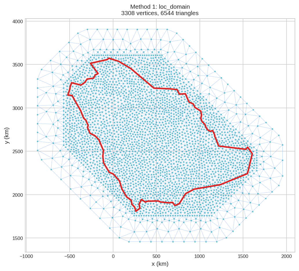
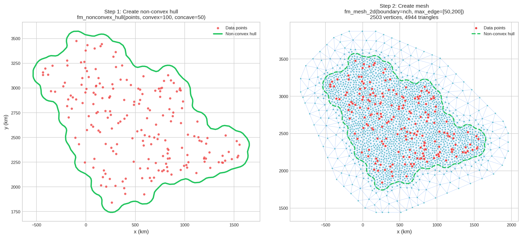
Method 2: Using fm_nonconvex_hull
Use fm_nonconvex_hull to create a smooth, simplified boundary from your country polygon:
# Extract boundary coordinates
boundary_coords = np.array(saudi_km.geometry.iloc[0].exterior.coords)

# Create non-convex hull around the boundary
nch_boundary = fm_nonconvex_hull(
    boundary_coords,
    convex=100,       # Convexity parameter (km)
    concave=50,      # Concavity parameter (km)
    resolution=[100, 90]  # Number of boundary points
)

# Create mesh with non-convex hull as boundary
mesh2 = fm_mesh_2d(
    boundary=nch_boundary,
    max_edge=[50, 200],
    offset=[0, 300],
    cutoff=25
)

print(f"Mesh has {mesh2.n} vertices")# Plot mesh with both boundaries
fig, ax = mesh2.plot(title="Method 2: fm_nonconvex_hull", show=False)
saudi_km.boundary.plot(ax=ax, color='red', linewidth=1.5, label='Country border')
# Plot the non-convex hull boundary
hull_pts = np.vstack([nch_boundary.loc, nch_boundary.loc[0]]) # Close the polygon
ax.plot(hull_pts[:, 0], hull_pts[:, 1], color='green', linewidth=2, linestyle='--', label='Non-convex hull')
ax.legend()
plt.show()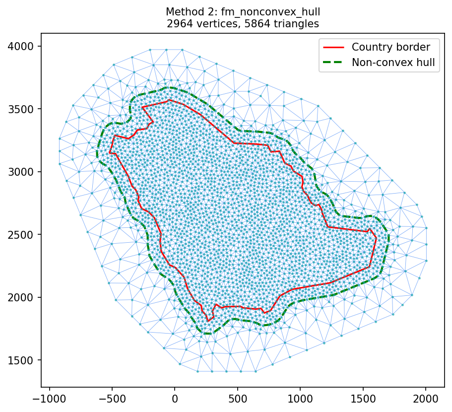
convex- How far the boundary can bulge outward (larger = smoother)concave- How far the boundary can indent inward (larger = smoother)resolution- Number of points defining the boundary (more = finer detail)
Understanding the Parameters
The three parameters control different aspects of the boundary shape:
convex - Outward bulge distance
Controls how far the boundary can extend outward from the data points. Larger values create smoother, more convex shapes:
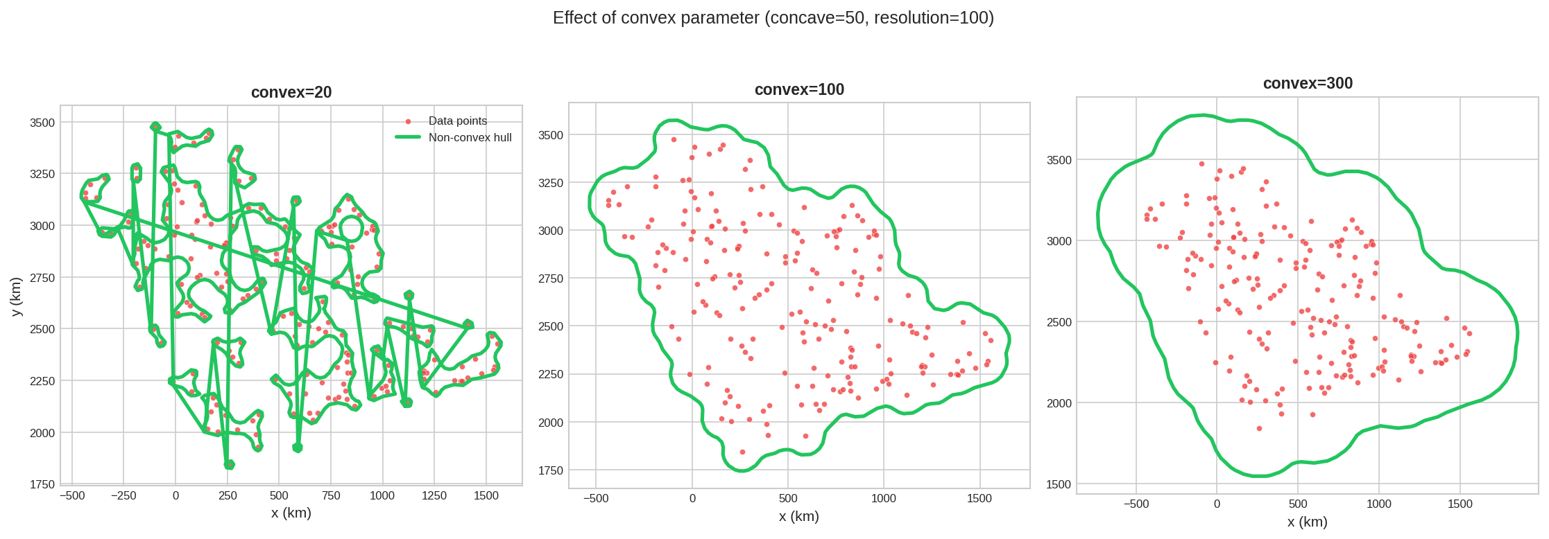
- Small convex (20): Tight boundary, closely following data point clusters
- Medium convex (100): Balanced smoothness
- Large convex (300): Very smooth boundary, may extend far beyond data
concave - Inward indent distance
Controls how far the boundary can indent inward into gaps between data points. Larger values prevent deep indentations:
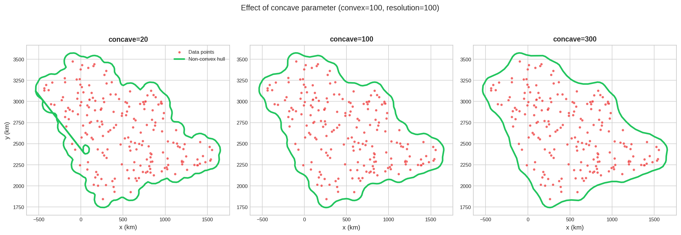
- Small concave (20): Allows deep indentations following gaps in data
- Medium concave (100): Moderate indentation, smoother boundary
- Large concave (300): Nearly no indentation, more convex overall
resolution - Number of boundary points
Controls how many points define the boundary. More points create finer detail but increase mesh complexity:
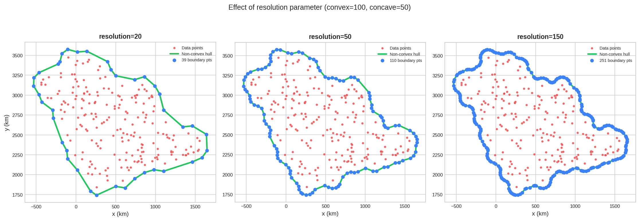
- Low resolution (20): Coarse boundary with 20 points, fast but may miss details
- Medium resolution (50): Good balance of detail and efficiency
- High resolution (150): Fine boundary detail, more mesh triangles needed
From Hull to Mesh
Once you have the non-convex hull, pass it as the boundary argument to fm_mesh_2d:
convex=concave (e.g., both 100) for balanced boundaries. Increase both for smoother shapes, decrease for tighter fits around your data.
Method 3: Using fm_hexagon_lattice
For uniform spatial coverage, use fm_hexagon_lattice to generate evenly-spaced points:
# Extract boundary coordinates
boundary_coords = np.array(saudi_km.geometry.iloc[0].exterior.coords)

# Generate hexagon lattice with 100 km buffer
hex_points = fm_hexagon_lattice(
    boundary_coords,
    edge_len=50,    # 50 km spacing between points
    geo_buffer=100  # 100 km buffer around boundary
)
print(f"Generated {len(hex_points)} hexagon lattice points")

# Create mesh from hexagon points
mesh3 = fm_mesh_2d(
    loc=hex_points,
    offset=500,       # Large outer extension
    max_edge=200      # Coarse outer triangles
)

print(f"Mesh has {mesh3.n} vertices")Mesh has 1466 vertices
# Plot mesh with country border and hex points
fig, ax = mesh3.plot(title="Method 3: fm_hexagon_lattice", show=False)
saudi_km.boundary.plot(ax=ax, color='red', linewidth=1.5)
ax.scatter(hex_points[:, 0], hex_points[:, 1], c='green', s=8, zorder=4)
plt.show()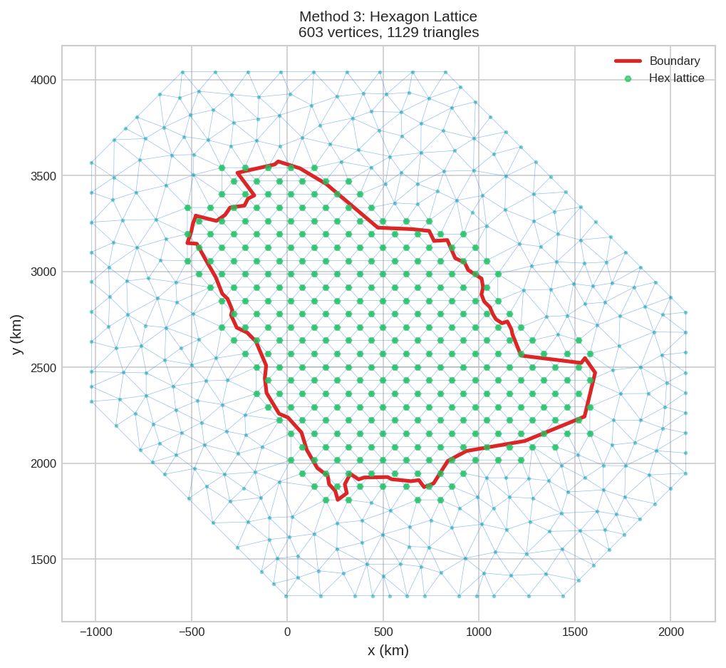
Choosing the Right Method
| Scenario | Recommended Method |
|---|---|
| You have exact study area boundary | Method 1: loc_domain |
| You have scattered observation points | Method 2: fm_nonconvex_hull |
| You need uniform prediction grid | Method 3: fm_hexagon_lattice |
| Complex coastline (many small features) | Method 2 or 3: Avoid tracing every detail |
| Prediction focus on specific subregions | Method 2: Hull adapts to data density |
offset and max_edge settings to avoid boundary artifacts. See Mesh Generation for parameter guidelines.