Spatial Temperature Modeling with SPDE
Build a spatial temperature model using SPDE (Stochastic Partial Differential Equations) with INLA. Fit the model with elevation as a covariate, visualize spatial effects, and generate predictions with uncertainty quantification.
By Esmail Abdul Fattah and Elias Krainski
The Statistical Model
We fit a spatial model for January 2024 average temperature:
Where:
- $\beta_0$: Intercept (baseline temperature at sea level)
- $\beta_1$: Elevation effect (temperature change per 1000m, expect ~-6 degrees C)
- $u(s)$: Spatial random effect (Matern Gaussian random field)
- $\varepsilon$: Observation noise
1. Setup and Imports
import numpy as np
import pandas as pd
import geopandas as gpd
import matplotlib.pyplot as plt
from matplotlib.tri import Triangulation
from scipy import stats
from shapely.geometry import Point
from shapely.ops import unary_union

# pyINLA imports
from pyinla import pyinla
from pyinla.fmesher import (
    fm_mesh_2d,
    fm_hexagon_lattice,
    spde2_pcmatern,
    spde_make_A,
    spde_grid_projector
)
2. Coordinate Reference System
For spatial modeling, we need projected coordinates (kilometers) rather than geographic coordinates (degrees):
# Coordinate Reference Systems
CRS_LONGLAT = "EPSG:4326"  # Standard WGS84 (degrees)
CRS_KM = "+proj=utm +zone=40 +ellps=intl +towgs84=-143,-236,7,0,0,0,0 +units=km +no_defs +type=crs"

# Study region
COUNTRIES = ["Lebanon", "Syria", "Jordan", "Saudi Arabia"]
This is essential because:
- The SPDE model assumes distances are in consistent units
- One degree of longitude varies in distance depending on latitude
- UTM Zone 40 is appropriate for the Middle East region
3. Load Temperature Data
We load the monthly temperature data from Part 1:
# Load temperature data from Part 1
tavg = pd.read_csv('tavg_month.csv')
print(f"Temperature data loaded: {tavg.shape[0]} stations")

# First 2 rows:
#        station  latitude  longitude  elevation  X202401  X202402  ...
# 0  BA000041150   26.2670      50.65        2.0    20.71    19.93  ...
# 1  IS000004640   32.9667      35.50      934.0     9.05     8.74  ...
Temperature data loaded: 55 stationsLoad country boundaries and project to the km-based CRS:
# Load country boundaries
NE_URL = "https://naciscdn.org/naturalearth/50m/cultural/ne_50m_admin_0_countries.zip"
worldMapll = gpd.read_file(NE_URL)
map_ll = worldMapll[worldMapll["ADMIN"].isin(COUNTRIES)].copy()
map2km = map_ll.to_crs(CRS_KM)
# Create station locations in km CRS
geometry = [Point(lon, lat) for lon, lat in zip(tavg["longitude"], tavg["latitude"])]
tavg_gdf = gpd.GeoDataFrame(tavg, geometry=geometry, crs=CRS_LONGLAT)
tavg_km = tavg_gdf.to_crs(CRS_KM)
coords_km = np.column_stack([tavg_km.geometry.x, tavg_km.geometry.y])
# Plot stations: color = temperature, size = elevation
fig, ax = plt.subplots(figsize=(10, 8))
map2km.boundary.plot(ax=ax, color='black', linewidth=1.5)
sc = ax.scatter(
coords_km[:, 0], coords_km[:, 1],
c=tavg['X202401'], cmap='RdYlBu_r',
s=tavg['elevation'] / 20 + 20,
edgecolors='black', linewidth=0.5, zorder=5
)
plt.colorbar(sc, ax=ax, shrink=0.7, label='January 2024 mean temperature (°C)')
ax.set_title('Weather stations: color = temperature, size = elevation')
ax.set_xlabel('Easting (km)')
ax.set_ylabel('Northing (km)')
ax.set_aspect('equal')
plt.tight_layout()
plt.show()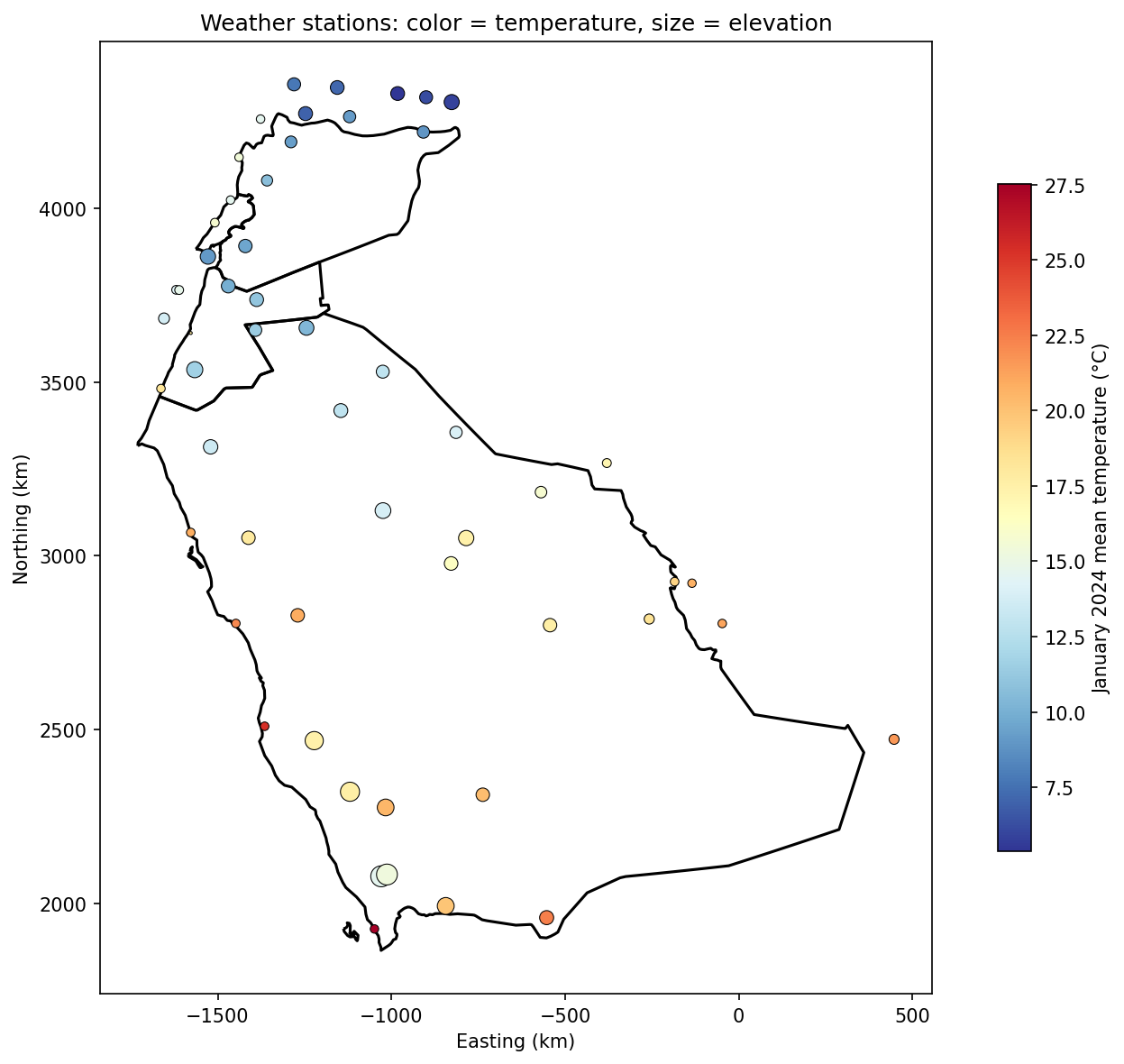
4. Check Elevation Effect
Before fitting the full spatial model, we verify that elevation affects temperature using simple linear regression:
valid = ~np.isnan(tavg['X202401']) & ~np.isnan(tavg['elevation'])
slope, intercept, r, p, se = stats.linregress(
    tavg.loc[valid, 'elevation'], tavg.loc[valid, 'X202401']
)

print(f"Slope (per 1000m): {slope*1000:.2f} °C/km")
print(f"R-squared: {r**2:.4f}")
Slope (per 1000m): -2.28 °C/km
R-squared: 0.0518What This Tells Us
- The negative slope confirms temperature decreases with elevation
- The magnitude (~2.3 degrees C per 1000m) is in the direction of the environmental lapse rate (~6.5 degrees C/km), but much weaker without a spatial effect
- The low R-squared indicates elevation alone doesn't explain all variation
- This motivates adding a spatial random effect
5. Create the Triangular Mesh
The SPDE approach requires a triangular mesh that covers the study region. The mesh serves as the computational domain for the spatial random field.
Mesh Construction Steps
- Buffer the boundary by 100 km (to avoid edge effects)
- Generate hexagonal lattice points (edge length = 50 km)
- Build triangular mesh with specified resolution
# Create unified boundary and buffer by 100 km
boundary = unary_union(map2km.geometry)
boundary_buffered = boundary.buffer(100)

# Extract boundary coordinates for hexagonal lattice
if boundary_buffered.geom_type == 'MultiPolygon':
    largest = max(boundary_buffered.geoms, key=lambda p: p.area)
    boundary_coords = np.array(largest.exterior.coords)
else:
    boundary_coords = np.array(boundary_buffered.exterior.coords)

# Create hexagonal lattice points
hexpoints = fm_hexagon_lattice(boundary_coords, edge_len=50)
print(f"Hexagonal lattice: {len(hexpoints)} points")

# Build the triangular mesh
mesh = fm_mesh_2d(
    loc=hexpoints,
    offset=500,     # Extend 500 km beyond boundary
    max_edge=200    # Maximum triangle edge: 200 km
)

print(f"Mesh: {mesh.n} vertices, {mesh.n_triangle} triangles")
Mesh: 1,792 vertices, 3,499 triangles# Plot mesh using built-in method
fig, ax = mesh.plot(locs=coords_km, title='SPDE Mesh', show=False)
map2km.boundary.plot(ax=ax, color='black', linewidth=2)
plt.tight_layout()
plt.show()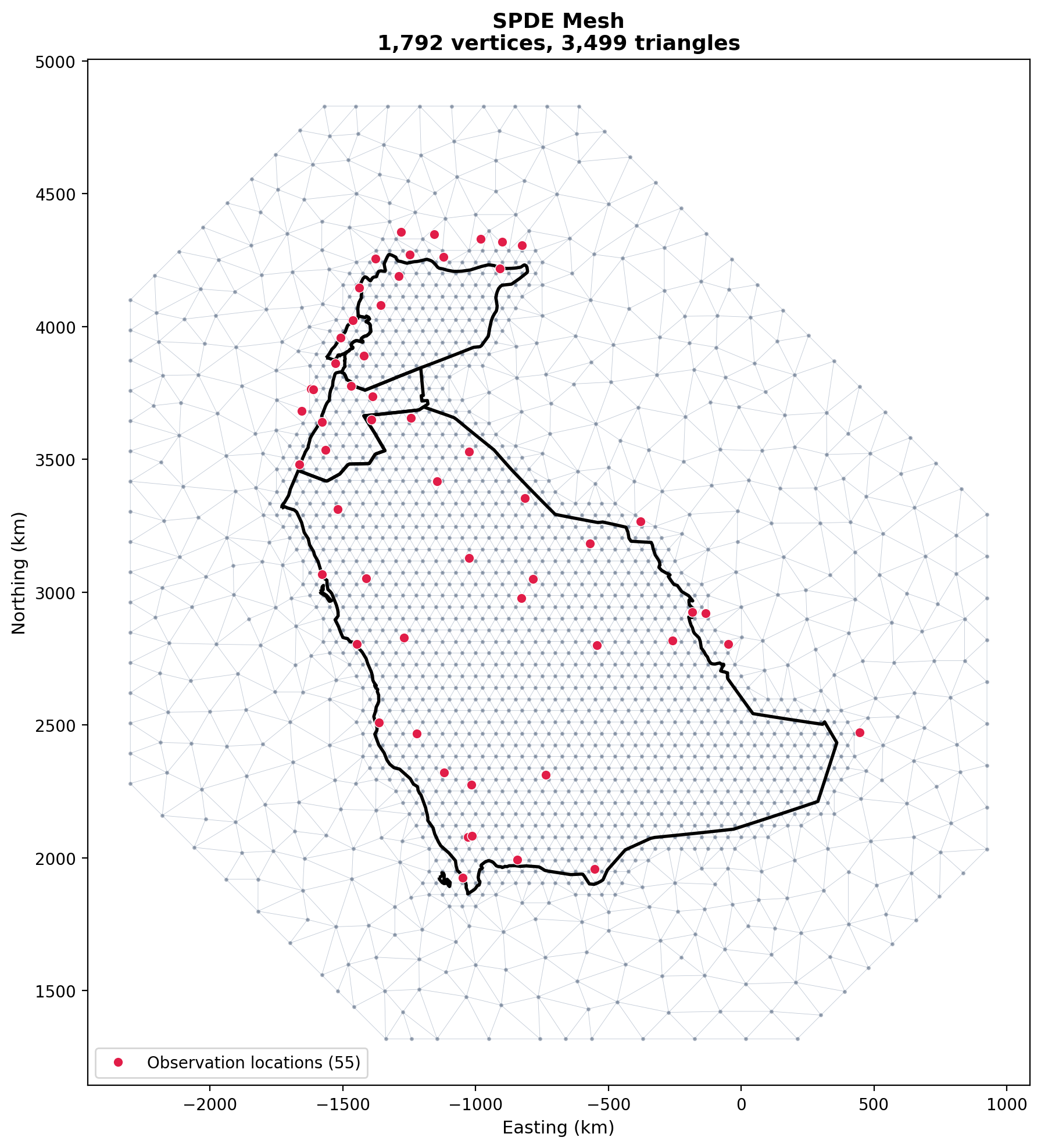
6. Define the SPDE Model
The SPDE model uses Penalized Complexity (PC) priors that shrink toward a base model:
| Prior | Specification | Interpretation |
|---|---|---|
| Range | P(range < 30 km) = 0.05 | We believe spatial correlation extends beyond 30 km |
| Sigma | P(sigma > 1 degrees C) = 0.05 | We believe spatial variation is typically less than 1 degrees C |
# Define SPDE model with PC priors
spdeModel = spde2_pcmatern(
    mesh=mesh,
    prior_range=(30, 0.05),   # P(range < 30 km) = 0.05
    prior_sigma=(1, 0.05)     # P(sigma > 1°C) = 0.05
)

# Create projector matrix from mesh to observation locations
Amap = spde_make_A(mesh=mesh, loc=coords_km)
print(f"Projector matrix A: {Amap.shape}")
Projector matrix A: (55, 1792)7. Fit the Model with pyINLA
# Prepare data for INLA
n_obs = len(tavg)
dataf = pd.DataFrame({
    'X202401': tavg['X202401'].values,
    'elevation_km': tavg['elevation'].values / 1000,
    'spatial': np.arange(n_obs)
})

# Define the model
model = {
    'response': 'X202401',
    'fixed': ['1', 'elevation_km'],
    'random': [{'id': 'spatial', 'model': spdeModel, 'A.local': Amap}]
}

# Fit the model
sfit = pyinla(model=model, family='gaussian', data=dataf, verbose=False)
8. Model Results
print(sfit.summary_fixed)
print(sfit.summary_hyperpar)
mean sd 0.025quant 0.5quant 0.975quant mode
(Intercept) 20.124107 3.872591 12.099176 20.123795 28.143617 20.123180
elevation_km -5.738761 0.370071 -6.466339 -5.739090 -5.009235 -5.739068
mean sd 0.025quant 0.5quant 0.975quant mode
Precision for the Gaussian observations 1.262697 0.335082 0.729446 1.220725 2.038849 1.141178
Range for spatial 2957.504758 901.562679 1570.932977 2829.684896 5085.210525 2590.809299
Stdev for spatial 2.801823 0.479452 1.981045 2.760177 3.863091 2.676366Fixed Effects
| Parameter | Mean | SD | 95% CI | Interpretation |
|---|---|---|---|---|
| Intercept ($\beta_0$) | 20.12 | 3.87 | [12.10, 28.14] | Baseline temperature at sea level (degrees C) |
| Elevation ($\beta_1$) | -5.74 | 0.37 | [-6.47, -5.01] | Temperature drops ~5.7 degrees C per 1000m |
The elevation coefficient is close to the environmental lapse rate (~6.5 degrees C/km).
Hyperparameters
| Parameter | Mean | SD | 95% CI | Description |
|---|---|---|---|---|
| Precision | 1.26 | 0.34 | [0.73, 2.04] | Observation noise (higher = less noise) |
| Range | 2,958 km | 902 km | [1,571, 5,085] | Practical correlation range |
| Stdev | 2.80 | 0.48 | [1.98, 3.86] | Marginal SD of spatial field (degrees C) |
Interpreting the Results
Range. The range represents the distance beyond which spatial correlation is essentially zero. Our estimated range is ~2,958 km, meaning stations farther apart than this are essentially independent.
Marginal standard deviation. The marginal standard deviation ($\sigma = 2.80$ degrees C) represents the spatially structured variation remaining after accounting for the fixed effects. Two locations at the same elevation could still differ in temperature by roughly $\pm 2.80$ degrees C due to their spatial position alone, driven by factors not captured by elevation (proximity to the coast, local climate patterns, desert conditions).
Precision for Gaussian observations. The precision ($\approx 1.26$) is the inverse of the variance of the residual noise. Converting gives a noise standard deviation of approximately $1/\sqrt{1.26} \approx 0.89$ degrees C, representing the unexplained variation remaining after accounting for both the fixed effects and the spatial random field (measurement noise or micro-scale local variation).
Spatial effect vs. noise. The spatial effect (2.80 degrees C) is much larger than the noise (0.89 degrees C), meaning the model captures most of the spatial structure in the data, leaving only a small residual. This is consistent with the high $R^2 \approx 0.97$.
PC priors. We control the tails of the prior distributions. For the range, we set $P(\text{range} < 30\text{ km}) = 0.05$, encoding our belief that the range is much larger than 30 km. For $\sigma$, we control the upper tail to prevent unrealistically large variance.
Mesh edge length must be smaller than the expected range. If the range is smaller than the triangle edge, neighboring mesh nodes become independent, meaning the mesh is too coarse to capture the spatial structure. The PC prior value for the range (30 km) is chosen to be slightly smaller than the mesh edge length (50 km) as a reference point. With the mesh edge at 50 km and the estimated range at ~3,000 km, we have a very fine mesh relative to the spatial correlation structure. We could increase the edge length to 100 km for faster computation without expecting much effect on the results, since the range is still far larger than the mesh resolution.
Fixed effect coefficients change with a spatial random effect. In our case, the elevation coefficient shifted from $-2.2$ to $-5.74$ degrees C per km, much closer to the known physical environmental lapse rate of ~6.5 degrees C/km. The spatial effect absorbed confounded variation and allowed the fixed effect to better reflect the true physical relationship.
Adapting mesh resolution to the variable. Temperature has a long range, so a coarser mesh may suffice. However, for rainfall we need to keep a fine mesh (50 km or even finer) because rainfall exhibits much more localized spatial variation: it can rain at only one station while surrounding stations remain dry, so the spatial correlation is much shorter and the mesh must be detailed enough to capture these rapid changes.
9. Model Fit
# Plot fitted vs observed
fitted_mean = sfit.summary_fitted_values['mean'].values
observed = tavg['X202401'].values
valid = ~np.isnan(observed)
r_sq = np.corrcoef(fitted_mean[valid], observed[valid])[0, 1] ** 2
print(f"R-squared: {r_sq:.4f}")
R-squared: 0.9788The $R^2 = 0.9788$ indicates the model (intercept + elevation + spatial random effect) explains nearly all of the observed temperature variation.
fig, ax = plt.subplots(figsize=(7, 7))
ax.scatter(fitted_mean[valid], observed[valid], marker='o', s=60,
           c='#3498db', alpha=0.7)
lims = [min(fitted_mean[valid].min(), observed[valid].min()) - 1,
        max(fitted_mean[valid].max(), observed[valid].max()) + 1]
ax.plot(lims, lims, 'r--', linewidth=2, label='Perfect fit')
ax.set_xlabel('Fitted (posterior mean, °C)')
ax.set_ylabel('Observed (°C)')
ax.set_title(f'Model fit: R² = {r_sq:.4f}')
ax.legend()
ax.grid(True, alpha=0.3)
plt.tight_layout()
plt.show()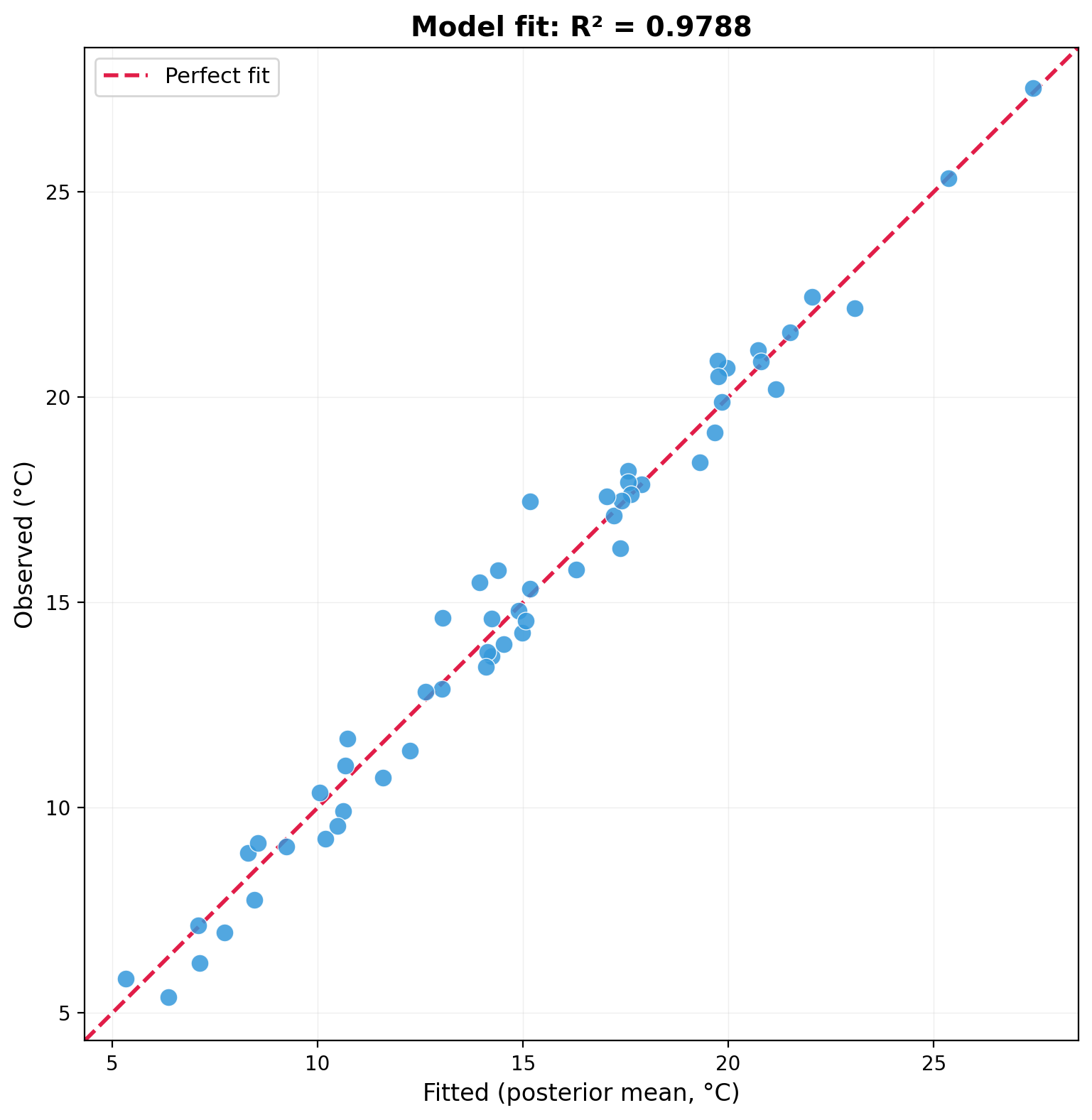
10. Create the Grid Projector
To visualize spatial fields on a regular grid, we create a grid projector that maps from mesh vertices to a 200 x 200 pixel grid covering the study region:
# Create grid projector for visualization
bb = map2km.total_bounds  # [minx, miny, maxx, maxy]
bb0_x = (bb[0], bb[2])
bb0_y = (bb[1], bb[3])

projGrid = spde_grid_projector(
    mesh=mesh,
    xlim=bb0_x,
    ylim=bb0_y,
    dims=(200, 200)
)
print(f"Grid projector: {projGrid.dims[0]}x{projGrid.dims[1]} = {projGrid.n_grid} points")
print(f"X range: {bb0_x[0]:.0f} to {bb0_x[1]:.0f} km")
print(f"Y range: {bb0_y[0]:.0f} to {bb0_y[1]:.0f} km")
Grid projector: 200x200 = 40000 points
X range: -1730 to 360 km
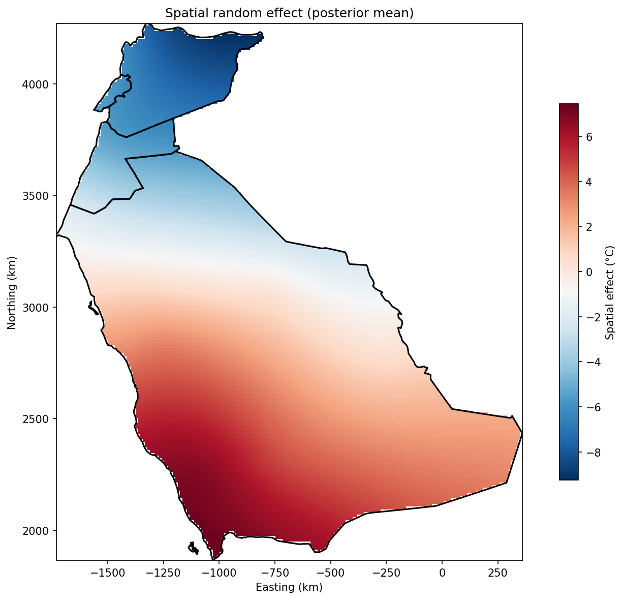
Y range: 1864 to 4272 km11. Visualize the Spatial Effect
The spatial random effect $u(s)$ captures geographic patterns not explained by elevation:
# Find grid points outside the country boundary
bnd = unary_union(map2km.geometry)
sfGrid = gpd.GeoDataFrame(
    geometry=gpd.points_from_xy(projGrid.lattice[:, 0], projGrid.lattice[:, 1]),
    crs=CRS_KM
)
igrid_out = ~sfGrid.within(bnd)

# Project spatial effect to grid
spatial_mean = sfit.summary_random['spatial']['mean'].values
gridSmean = projGrid.project(spatial_mean, mask_outside=False)
gridSmean[igrid_out.values.reshape(projGrid.dims[1], projGrid.dims[0])] = np.nan

# Plot spatial effect
fig, ax = plt.subplots(figsize=(10, 8))
im = ax.imshow(
    gridSmean, origin='lower',
    extent=[bb0_x[0], bb0_x[1], bb0_y[0], bb0_y[1]],
    cmap='RdBu_r', aspect='equal'
)
map2km.boundary.plot(ax=ax, color='black', linewidth=1.5)
plt.colorbar(im, ax=ax, shrink=0.7, label='Spatial effect (°C)')
ax.set_title('Spatial random effect (posterior mean)')
ax.set_xlabel('Easting (km)')
ax.set_ylabel('Northing (km)')
plt.tight_layout()
plt.show()
What This Tells Us
- Positive values (red): Warmer than expected based on elevation alone
- Negative values (blue): Cooler than expected
This captures regional climate patterns like coastal effects, continental effects, and local topographic effects.
12. Load Elevation Data (ETOPO)
To make predictions across the entire region, we need elevation at every grid point. We use ETOPO 2022 from NOAA via OpenDAP:
import xarray as xr

# Transform grid points back to lon/lat for ETOPO lookup
sfGrid_ll = sfGrid.to_crs(CRS_LONGLAT)
glocs = np.column_stack([sfGrid_ll.geometry.x, sfGrid_ll.geometry.y])

# Get bounding box in lon/lat (with some padding)
lon_min, lon_max = glocs[:, 0].min() - 1, glocs[:, 0].max() + 1
lat_min, lat_max = glocs[:, 1].min() - 1, glocs[:, 1].max() + 1

# Load ETOPO elevation data via OpenDAP
ETOPO_URL = "https://www.ngdc.noaa.gov/thredds/dodsC/global/ETOPO2022/60s/60s_surface_elev_netcdf/ETOPO_2022_v1_60s_N90W180_surface.nc"

ds = xr.open_dataset(ETOPO_URL, engine='netcdf4')
etopo = ds['z'].sel(
    lon=slice(lon_min, lon_max),
    lat=slice(lat_min, lat_max)
)

# Interpolate elevation at each grid point location
etopoll = etopo.interp(
    lon=xr.DataArray(glocs[:, 0], dims='points'),
    lat=xr.DataArray(glocs[:, 1], dims='points'),
    method='nearest'
).values

# Mask grid points outside the boundary
etopoll[igrid_out.values] = np.nan
ETOPO provides:
- Global coverage (land elevation + ocean depth)
- 1 arc-minute resolution (~1.8 km)
- Streaming access, no download required
13. Predictions with Uncertainty
A key advantage of Bayesian spatial models is uncertainty quantification. We append NA-response rows for each grid point so INLA predicts at those locations, then re-evaluate at the fitted mode (fast, no re-optimization):
from scipy import sparse

n_grid = projGrid.n_grid

# Prediction data: NA response so it will be predicted
preddf = pd.DataFrame({
    'X202401': np.full(n_grid, np.nan),
    'elevation_km': etopoll / 1000,
    'spatial': np.arange(n_obs, n_obs + n_grid)
})

# Combine observation + prediction data
data_combined = pd.concat([dataf, preddf], ignore_index=True)

# Combined projector matrix (observations + grid)
A_combined = sparse.vstack([Amap, projGrid.proj])

# Model with combined A matrix
model_pred = {
    'response': 'X202401',
    'fixed': ['1', 'elevation_km'],
    'random': [{'id': 'spatial', 'model': spdeModel, 'A.local': A_combined}]
}

# Re-fit at the fitted mode (fast, no optimization)
sfit_pred = pyinla(
    model=model_pred,
    family='gaussian',
    data=data_combined,
    control={'mode': {'theta': sfit.mode['theta'], 'restart': False}},
    verbose=False
)

# Extract predictions for the grid points
i_pred = slice(n_obs, n_obs + n_grid)
pred_mean = sfit_pred.summary_fitted_values['mean'].values[i_pred]
pred_sd = sfit_pred.summary_fitted_values['sd'].values[i_pred]

# Reshape to grid and mask outside boundary
igrid_out_2d = igrid_out.values.reshape(projGrid.dims[1], projGrid.dims[0])

pred_grid = pred_mean.reshape(projGrid.dims[1], projGrid.dims[0])
pred_grid[igrid_out_2d] = np.nan

sd_pred_grid = pred_sd.reshape(projGrid.dims[1], projGrid.dims[0])
sd_pred_grid[igrid_out_2d] = np.nan
14. Final Results
The model produces two key outputs:
Predicted Temperature (Posterior Mean)
- Warmest: Low-elevation Saudi Arabian desert (~25-28 degrees C)
- Coolest: Mountains of Lebanon and Syria (~5-10 degrees C)
- Clear elevation-driven gradient across the region
Prediction Uncertainty (Posterior SD)
- Lowest uncertainty: Near weather stations (direct information)
- Higher uncertainty: Data-sparse areas (interior Saudi Arabia)
- Range: 0.38 to 1.46 degrees C
This uncertainty map is valuable for planning where additional monitoring would be most beneficial.
# Plot prediction and uncertainty side by side
fig, axes = plt.subplots(1, 2, figsize=(14, 6))

# Left: Predicted temperature
ax = axes[0]
im1 = ax.imshow(
    pred_grid, origin='lower',
    extent=[bb0_x[0], bb0_x[1], bb0_y[0], bb0_y[1]],
    cmap='RdYlBu_r', aspect='equal'
)
map2km.boundary.plot(ax=ax, color='black', linewidth=1.5)
plt.colorbar(im1, ax=ax, shrink=0.7, label='Temperature (°C)')
ax.set_title('(a) Predicted temperature (posterior mean)')
ax.set_xlabel('Easting (km)')
ax.set_ylabel('Northing (km)')

# Right: Uncertainty with stations
ax = axes[1]
im2 = ax.imshow(
    sd_pred_grid, origin='lower',
    extent=[bb0_x[0], bb0_x[1], bb0_y[0], bb0_y[1]],
    cmap='YlOrRd', aspect='equal'
)
map2km.boundary.plot(ax=ax, color='black', linewidth=1.5)
ax.scatter(coords_km[:, 0], coords_km[:, 1],
           marker='o', s=40, c='black', zorder=5, label='Weather stations')
plt.colorbar(im2, ax=ax, shrink=0.7, label='SD (°C)')
ax.set_title('(b) Prediction uncertainty')
ax.set_xlabel('Easting (km)')
ax.set_ylabel('Northing (km)')
ax.legend(loc='upper right', fontsize=9)

plt.tight_layout()
plt.show()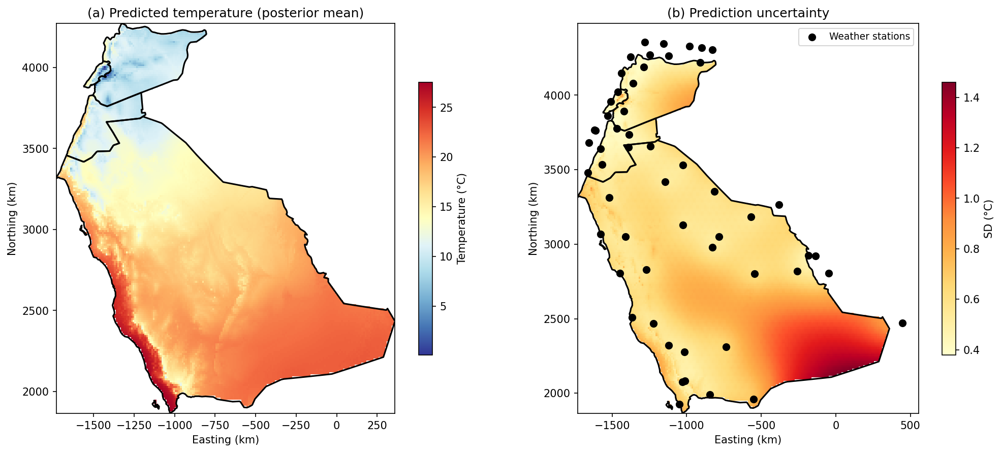
A Note on High Uncertainty in the Southeast
Notice the elevated prediction uncertainty (SD > 1 degrees C) in the southeastern part of Saudi Arabia. This is a classic boundary effect in spatial modeling: predictions become less reliable at the edges of the study region where:
- No nearby stations exist to anchor the spatial field
- The model extrapolates rather than interpolates
- The mesh boundary influences the spatial random effect
This high uncertainty is not a bug. It is the model honestly reporting that predictions in this area are less reliable.
Challenges for the Reader
Challenge 1: Model Summer Temperatures
This application modeled January (X202401), a winter month. How do temperature patterns change in summer?
Try modeling July (X202407):
- Change the response variable from
'X202401'to'X202407' - Re-fit the model and compare results
- Questions to explore:
- How does the intercept ($\beta_0$) change? (Expect much higher!)
- Does the elevation effect ($\beta_1$) change?
- How do spatial patterns differ between winter and summer?
- Where are the hottest predicted temperatures?
Challenge 2: Reduce Boundary Uncertainty
Can you reduce the prediction uncertainty in southeastern Saudi Arabia?
Hint: Add weather stations from Oman to your dataset. Oman borders Saudi Arabia to the southeast and has GHCN stations with TAVG data.
Steps:
- Go back to Part 1 and modify
COUNTRIESto include"Oman" - Re-run the data collection to get stations from Oman
- Re-fit the spatial model with the expanded dataset
- Compare the uncertainty maps: the southeastern boundary should improve!
This exercise demonstrates a key principle: spatial models benefit from data beyond the prediction boundary.
Summary
| Component | Value |
|---|---|
| Study Region | Lebanon, Syria, Jordan, Saudi Arabia |
| Stations | 55 |
| Response | X202401 (January 2024 mean temperature) |
| Mesh | 1,792 vertices, 3,499 triangles |
| Intercept ($\beta_0$) | 20.12 degrees C (sea level temperature) |
| Elevation ($\beta_1$) | -5.74 degrees C per 1000m |
| Model R-squared | 0.9788 |
| Prediction Grid | 200 x 200 = 40,000 points |
| Temperature Range | -2.5 to 27.7 degrees C |
| Uncertainty Range | 0.38 to 1.46 degrees C |
Key Takeaways
- SPDE provides efficient spatial modeling: Matern fields via triangular mesh
- PC priors encode prior beliefs: Range and sigma specifications
- The projector matrix A connects mesh to observations
- Elevation explains much variation: $\beta_1 \approx$ -5.7 degrees C/km matches lapse rate
- Spatial effect captures residual patterns: Coastal vs. continental effects
- Uncertainty quantification is automatic: Lower near stations, higher elsewhere
- pyINLA syntax is straightforward: Dict-based model specification
References
- Lindgren, F., Rue, H., and Lindstrom, J. (2011). "An explicit link between Gaussian fields and Gaussian Markov random fields: the stochastic partial differential equation approach." Journal of the Royal Statistical Society: Series B, 73(4), 423-498.
- Fuglstad, G.-A., Simpson, D., Lindgren, F., and Rue, H. (2019). "Constructing Priors that Penalize the Complexity of Gaussian Random Fields." Journal of the American Statistical Association, 114(525), 445-452.
- GHCN-Daily: Menne, M.J., et al. (2012). "Global Historical Climatology Network - Daily." NOAA National Climatic Data Center.