SPDE Application · Part 1

Collecting Temperature Data for Spatial Modeling

Download and prepare weather station data from the Global Historical Climatology Network (GHCN) for spatial temperature modeling over Lebanon, Syria, Jordan, and Saudi Arabia.

By Esmail Abdul Fattah and Elias Krainski

What We'll Build

By the end of this walkthrough, you'll have:

Downloaded global weather station metadata and daily observations
Filtered stations within our study region (100 km buffer)
Created three output files for spatial analysis:
- tavg_day.csv - Daily average temperatures
- tavg_month.csv - Monthly average temperatures
- tavg.csv - Weekly averages for summer weeks (21-34)

The Data Source: GHCN-Daily

GHCN-Daily is one of the most comprehensive global weather datasets, maintained by NOAA. It contains:

100,000+ stations worldwide
Daily observations including temperature, precipitation, snow
Quality-controlled data going back to the 1800s

We use the TAVG (average temperature) element, which provides daily mean temperature in tenths of degrees Celsius.

1. Setup and Configuration

First, we import the required libraries and set our configuration parameters:

import gzip
import urllib.request
from pathlib import Path

import numpy as np
import pandas as pd
import geopandas as gpd
import matplotlib.pyplot as plt
from shapely.geometry import Point
from shapely.ops import unary_union

# Configuration
DATA_DIR = Path(".")
YEAR = 2024
COUNTRIES = ["Lebanon", "Syria", "Jordan", "Saudi Arabia"]
DISTANCE_M = 1e5  # 100 km buffer around the study region

Key settings:

YEAR: Which year of data to analyze (2024)
COUNTRIES: Our study region covering the eastern Mediterranean and Arabian Peninsula
DISTANCE_M: Buffer distance around the region (100 km) to capture nearby stations

2. Download GHCN Data Files

We need two files from NOAA's GHCN repository:

File	Description	Size
`ghcnd-stations.txt`	Metadata for ~130,000 stations	~10 MB
`2024.csv.gz`	All daily observations for 2024	~2 GB compressed

GHCN_URL = "https://www.ncei.noaa.gov/pub/data/ghcn/daily"

for filename, url in [
    ("ghcnd-stations.txt", f"{GHCN_URL}/ghcnd-stations.txt"),
    (f"{YEAR}.csv.gz", f"{GHCN_URL}/by_year/{YEAR}.csv.gz")
]:
    path = DATA_DIR / filename
    if not path.exists():
        print(f"Downloading {filename}...")
        urllib.request.urlretrieve(url, path)
    else:
        print(f"[SKIP] {filename} already exists")

3. Load Station Metadata

The station file uses a fixed-width format. We extract:

station: 11-character unique identifier
latitude/longitude: Geographic coordinates (WGS84)
elevation: Height above sea level in meters

# Read station metadata (fixed-width format)
stations = pd.read_fwf(
    DATA_DIR / "ghcnd-stations.txt",
    colspecs=[(0,11), (12,20), (21,30), (31,37), (38,40), (41,71)],
    names=["station", "latitude", "longitude", "elevation", "state", "name"],
    dtype={"station": str}
)
stations["station"] = stations["station"].str.strip()

# Convert to GeoDataFrame
geometry = [Point(lon, lat) for lon, lat in zip(stations["longitude"], stations["latitude"])]
allst = gpd.GeoDataFrame(stations, geometry=geometry, crs="EPSG:4326")

print(f"Total stations in GHCN database: {len(allst):,}")

Total stations in GHCN database: 129,657

4. Load and Filter Temperature Data

The yearly data file contains all observation types. We filter for TAVG only and convert to degrees Celsius:

with gzip.open(DATA_DIR / f"{YEAR}.csv.gz", "rt") as f:
    df = pd.read_csv(
        f, header=None,
        names=["station", "date", "element", "value", "mflag", "qflag", "sflag", "obstime"],
        dtype={"station": str, "date": str},
        usecols=["station", "date", "element", "value"]
    )

# Filter TAVG and convert to degrees Celsius
tavg_df = df[df["element"] == "TAVG"].copy()
tavg_df["value"] = tavg_df["value"] / 10.0  # GHCN stores in tenths of degrees

# Pivot to wide format (stations x dates)
wd0 = tavg_df.pivot(index="station", columns="date", values="value")

Note: GHCN stores temperatures in tenths of degrees C, so we divide by 10.

5. Load Study Region Boundaries

We load country boundaries from Natural Earth, a free public domain map dataset:

# Load country boundaries from Natural Earth
NE_URL = "https://naciscdn.org/naturalearth/50m/cultural/ne_50m_admin_0_countries.zip"
world = gpd.read_file(NE_URL)
map_gdf = world[world["ADMIN"].isin(COUNTRIES)]

print(f"Loaded countries: {list(map_gdf['ADMIN'])}")

Loaded countries: ['Syria', 'Saudi Arabia', 'Lebanon', 'Jordan']

# Plot study region
fig, ax = plt.subplots(figsize=(10, 8))
map_gdf.plot(ax=ax, color='#e5e7eb', edgecolor='black', linewidth=1.5)
for _, row in map_gdf.iterrows():
    centroid = row.geometry.centroid
    ax.text(centroid.x, centroid.y, row['ADMIN'], ha='center', fontsize=10, fontweight='bold')
ax.set_title('Study Region: Lebanon, Syria, Jordan, Saudi Arabia')
ax.set_xlabel('Longitude')
ax.set_ylabel('Latitude')
plt.tight_layout()
plt.show()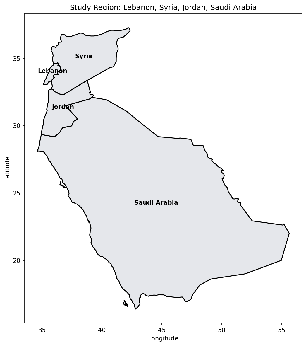

Study region map showing Lebanon, Syria, Jordan, and Saudi Arabia — Study region: Lebanon, Syria, Jordan, and Saudi Arabia

6. Select Stations Within Study Region

We select all stations within 100 km of our country boundaries. This buffer ensures we capture stations near the borders that may provide useful spatial information.

# Create unified boundary
boundary = unary_union(map_gdf.geometry)

# Project to UTM for accurate distance calculation
allst_proj = allst.to_crs("EPSG:32637")
boundary_proj = gpd.GeoSeries([boundary], crs="EPSG:4326").to_crs("EPSG:32637").iloc[0]

# Find stations within distance threshold
ii = allst_proj.distance(boundary_proj) <= DISTANCE_M

# Check which of these have TAVG data
ii_d = allst.loc[ii, "station"].isin(wd0.index)

print(f"Stations within {DISTANCE_M/1000:.0f} km of boundary: {ii.sum()}")
print(f"Stations with {YEAR} TAVG data: {ii_d.sum()}")

Stations within 100 km of boundary: 84
Stations with 2024 TAVG data: 55

# Plot station coverage
fig, ax = plt.subplots(figsize=(10, 8))
map_gdf.plot(ax=ax, color='#e5e7eb', edgecolor='black', linewidth=1.5)

# Stations in range without TAVG data
no_data = allst.loc[ii & ~ii_d]
ax.scatter(no_data.geometry.x, no_data.geometry.y,
           marker='o', s=30, c='blue', alpha=0.5, label='No TAVG data')

# Stations in range with TAVG data
with_data = allst.loc[ii & ii_d]
ax.scatter(with_data.geometry.x, with_data.geometry.y,
           marker='o', s=50, c='red', zorder=5, label=f'With TAVG ({ii_d.sum()} stations)')

ax.set_title(f'Station Coverage: {ii_d.sum()} stations with TAVG data')
ax.set_xlabel('Longitude')
ax.set_ylabel('Latitude')
ax.legend(loc='lower left')
plt.tight_layout()
plt.show()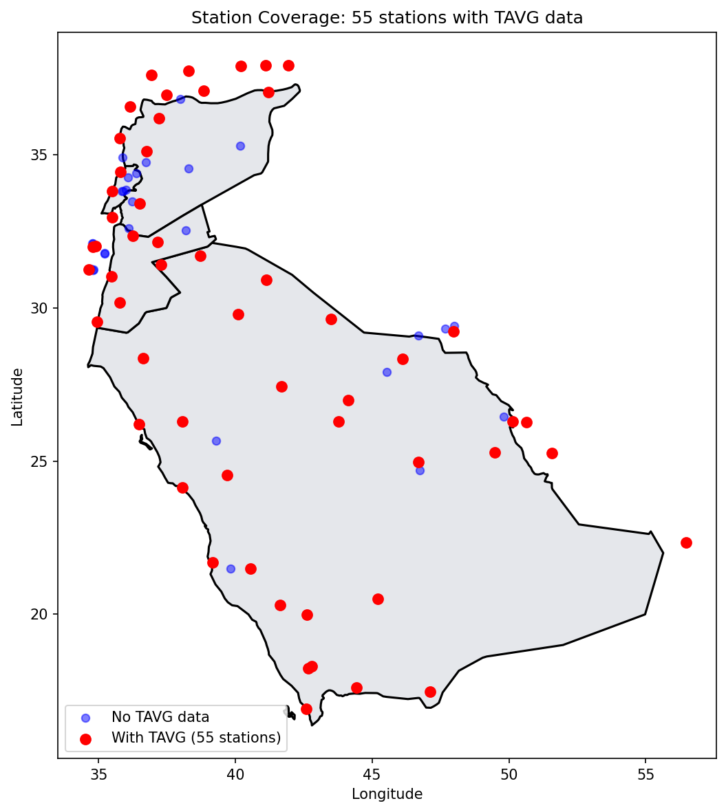

Weather station coverage in the study region — Weather stations with TAVG data within 100 km of the study region boundary

What This Tells Us

Not all stations within our region have temperature data for the selected year
Some stations may only report precipitation or other variables
The spatial coverage affects our model's ability to capture local variations
Areas with sparse station coverage will have higher prediction uncertainty

7. Prepare Data for Export

Before creating output files, we extract the station metadata, temperature subset, and date index for the stations that have TAVG data:

# Get station IDs with data
station_ids_in_range = allst.loc[ii, "station"].tolist()
id_with_data = [s for s in station_ids_in_range if s in wd0.index]

# Parse dates
dates = pd.to_datetime(wd0.columns, format="%Y%m%d")

# Get station metadata for stations with data
stations_with_data = allst[allst["station"].isin(id_with_data)][
    ["station", "latitude", "longitude", "elevation"]
].copy()

# Get temperature subset
tavg_subset = wd0.loc[id_with_data]

print(f"Stations: {len(id_with_data)}")
print(f"Date range: {dates.min().date()} to {dates.max().date()}")
print(f"Days: {len(dates)}")

Stations: 55
Date range: 2024-01-01 to 2024-12-31
Days: 366

8. Create Output Files

We create three output files with different temporal aggregations:

8.1 Daily Temperatures (`tavg_day.csv`)

Contains daily average temperatures for all 366 days. Useful for time series analysis.

tavg_day = stations_with_data.copy().reset_index(drop=True)
for col in tavg_subset.columns:
    tavg_day[col] = tavg_subset[col].values.round(2)

tavg_day.to_csv(DATA_DIR / "tavg_day.csv", index=False)

8.2 Monthly Temperatures (`tavg_month.csv`)

Monthly averages are more stable for spatial modeling, smoothing out day-to-day variability:

tavg_values = tavg_subset.values
months = [col[:6] for col in tavg_subset.columns]  # Extract YYYYMM
unique_months = sorted(set(months))

tavg_month = stations_with_data.copy().reset_index(drop=True)
for month in unique_months:
    month_mask = [m == month for m in months]
    month_data = tavg_values[:, month_mask]
    tavg_month[f"X{month}"] = np.round(np.nanmean(month_data, axis=1), 2)

tavg_month.to_csv(DATA_DIR / "tavg_month.csv", index=False)

8.3 Weekly Summer Temperatures (`tavg.csv`)

Weekly averages for weeks 21-34 (mid-May to late August), the warmest period with most consistent data:

weeks = [d.strftime("%V") for d in dates]  # ISO week numbers
unique_weeks = sorted(set(weeks))
selected_weeks = [w for w in unique_weeks if 21 <= int(w) <= 34]

tavg_weekly = stations_with_data.copy().reset_index(drop=True)
for week in selected_weeks:
    week_mask = [w == week for w in weeks]
    week_data = tavg_values[:, week_mask]
    tavg_weekly[f"X{week}"] = np.round(np.nanmean(week_data, axis=1), 2)

tavg_weekly.to_csv(DATA_DIR / "tavg.csv", index=False)

Summary

We have successfully collected and prepared temperature data for spatial modeling:

Output File	Contents	Use Case
`tavg_day.csv`	Daily temperatures (366 days)	Time series analysis
`tavg_month.csv`	Monthly averages (12 months)	Spatial modeling (Part 2)
`tavg.csv`	Weekly summer averages (14 weeks)	Seasonal analysis

Next Steps

In Part 2, we will:

Build a triangular mesh over the study region
Define an SPDE spatial model with PC priors
Fit the model using pyINLA
Create temperature predictions with uncertainty maps

The tavg_month.csv file will be our primary input, using X202401 (January 2024) as the response variable.

Continue to Part 2: Spatial Modeling →