Premier League Match Prediction
How do we estimate team strength and predict match outcomes? Using a Bayesian Poisson GLMM with crossed random effects, we decompose football performance into attack and defense components, quantify home advantage, and simulate the final league table with full uncertainty.
Interpretable Insights from This Analysis
The Poisson GLMM decomposes match outcomes into interpretable components, each with quantified uncertainty:
| Component | Parameter | Football Insight |
|---|---|---|
| Home advantage | $\beta$ (home effect) | Playing at home increases expected goals by ~27% |
| Attack strength | $a_i$ (attack random effect) | Man City and Liverpool have the strongest attacks |
| Defensive strength | $d_j$ (defense random effect) | Lower values indicate fewer goals conceded |
| Season simulation | Posterior predictive | Probabilistic league table with top-4 and relegation odds |
Unlike deterministic ranking systems, this Bayesian approach provides full posterior distributions over team abilities, enabling principled uncertainty quantification for predictions.
Why Model Football with a Poisson GLMM?
Football match scores are counts (0, 1, 2, ...), making Poisson regression a natural choice. The key modeling decisions are:
- Crossed random effects: each observation is influenced by both the attacking team and the defending team. This structure (Dixon and Coles, 1997) separates team quality into offensive and defensive components.
- Home advantage: a fixed effect capturing the well-documented benefit of playing at home.
- Bayesian estimation: pyINLA provides fast, accurate posterior approximations with full uncertainty quantification.
This approach has been widely used in sports analytics for ranking teams, predicting match outcomes, and simulating tournament results.
About the Data
The dataset contains all scheduled matches from the English Premier League 2018-2019 season. Each match contributes two observations (one per team) to the model in long format.
- 20 teams, 380 scheduled matches
- 313 played matches (67 remaining are simulated for prediction)
- 626 observations in long format (2 per match)
| Variable | Description |
|---|---|
goals | Goals scored by the focal team |
attack | Team ID of the scoring team (1-20) |
defense | Team ID of the opposing team (1-20) |
home | 1 if the focal team is at home, 0 otherwise |
Download the data: PremierLeague.txt
import numpy as np
import pandas as pd

# Load match schedule from PremierLeague.txt
matches = []
with open('PremierLeague.txt', 'r') as f:
    for line in f:
        line = line.strip()
        if not line:
            continue
        parts = line.split()
        if len(parts) >= 5:
            home_team, away_team = parts[0], parts[1]
            home_goals, away_goals = parts[2], parts[4]
            if home_goals == 'NA':
                home_goals, away_goals = np.nan, np.nan
            else:
                home_goals, away_goals = int(home_goals), int(away_goals)
            matches.append({'home_team': home_team, 'away_team': away_team,
                            'home_goals': home_goals, 'away_goals': away_goals})

matches_df = pd.DataFrame(matches)

# Build team mappings (alphabetical, 1-indexed)
teams = sorted(matches_df['home_team'].unique())
team_to_id = {team: i + 1 for i, team in enumerate(teams)}
id_to_team = {v: k for k, v in team_to_id.items()}

# Split played vs unplayed (unplayed have NaN goals)
played_df = matches_df[matches_df['home_goals'].notna()].copy()

print(f"Teams: {len(teams)}")
print(f"Total matches: {len(matches_df)}")
print(f"Played: {len(played_df)}, Unplayed: {len(matches_df) - len(played_df)}")
Teams: 20
Total matches: 380
Played: 313, Unplayed: 67# Parse match data into long format
# Each match produces 2 rows: one for the home team, one for the away team
rows = []
for _, match in played_df.iterrows():
rows.append({
'goals': int(match['home_goals']),
'attack': team_to_id[match['home_team']],
'defense': team_to_id[match['away_team']],
'home': 1
})
rows.append({
'goals': int(match['away_goals']),
'attack': team_to_id[match['away_team']],
'defense': team_to_id[match['home_team']],
'home': 0
})
model_df = pd.DataFrame(rows)
print(f"Model data: {len(model_df)} rows ({len(played_df)} matches x 2)")
print(f"Mean goals per team per match: {model_df['goals'].mean():.2f}")Model data: 626 rows (313 matches x 2)
Mean goals per team per match: 1.42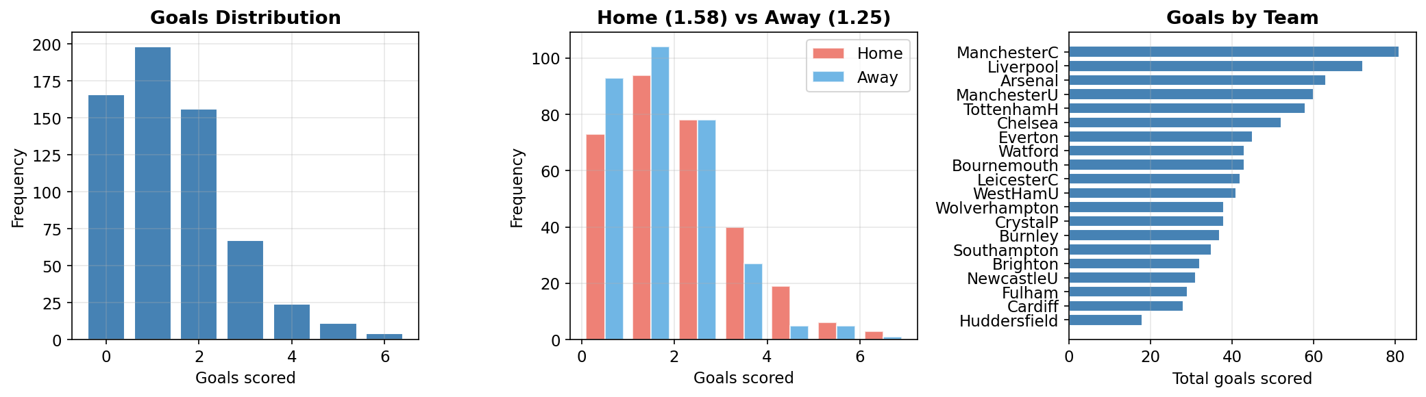
The Statistical Model
For each team-in-match observation, the number of goals follows a Poisson distribution:
where $a_i$ is the attack random effect for team $i$ (how many goals they tend to score) and $d_j$ is the defense random effect for team $j$ (how many goals they tend to concede). A positive $d_j$ means team $j$ concedes more goals than average.
Model Components
| Parameter | Description | Prior |
|---|---|---|
| $\mu$ (Intercept) | Baseline log-rate of goals | Default (flat) |
| $\beta$ (Home) | Home advantage on log scale | Default (flat) |
| $a_i$ (Attack) | IID random effects, $a_i \sim N(0, \tau_a^{-1})$ | $\tau_a \sim \text{LogGamma}(1, 0.01)$ |
| $d_j$ (Defense) | IID random effects, $d_j \sim N(0, \tau_d^{-1})$ | $\tau_d \sim \text{LogGamma}(1, 0.01)$ |
The crossed structure means each observation depends on two different grouping factors (attack team and defense team), unlike nested random effects. This is analogous to a two-way ANOVA with random row and column effects.
Step 1: Fit the Model with pyINLA
from pyinla import pyinla

model = {
    'response': 'goals',
    'fixed': ['1', 'home'],
    'random': [
        {'id': 'attack', 'model': 'iid',
         'hyper': {'prec': {'prior': 'loggamma', 'param': [1, 0.01], 'initial': 4}}},
        {'id': 'defense', 'model': 'iid',
         'hyper': {'prec': {'prior': 'loggamma', 'param': [1, 0.01], 'initial': 4}}}
    ]
}

result = pyinla(
    model=model,
    family='poisson',
    data=model_df,
    control={'compute': {'dic': True, 'mlik': True, 'return_marginals': True, 'config': True}},
    keep=True
)

print("Fixed effects:")
print(result.summary_fixed[['mean', 'sd', '0.025quant', '0.975quant']])
print("\nHyperparameters:")
print(result.summary_hyperpar[['mean', 'sd', '0.025quant', '0.975quant']])
Fixed effects:
mean sd 0.025quant 0.975quant
(Intercept) 0.150466 0.100775 -0.050613 0.346319
home 0.237082 0.067770 0.104192 0.369971
Hyperparameters:
mean sd 0.025quant 0.975quant
Precision for attack 12.408059 5.102967 5.216363 24.937421
Precision for defense 22.751188 11.569975 8.076033 52.307172Step 2: Interpret the Results
Home Advantage
The home effect $\beta \approx 0.24$ on the log scale corresponds to a multiplicative factor:
Playing at home increases the expected number of goals by approximately 27%. This is consistent with the well-documented home advantage in football.
home_effect = result.summary_fixed.loc['home', 'mean']
home_mult = np.exp(home_effect)
print(f"Home effect (log scale): {home_effect:.4f}")
print(f"Multiplicative effect: {home_mult:.3f}")
print(f"Playing at home increases expected goals by ~{(home_mult-1)*100:.0f}%")

intercept = result.summary_fixed.loc['(Intercept)', 'mean']
print(f"\nBaseline (away) goal rate: {np.exp(intercept):.3f}")
print(f"Home goal rate: {np.exp(intercept + home_effect):.3f}")
Home effect (log scale): 0.2371
Multiplicative effect: 1.268
Playing at home increases expected goals by ~27%
Baseline (away) goal rate: 1.162
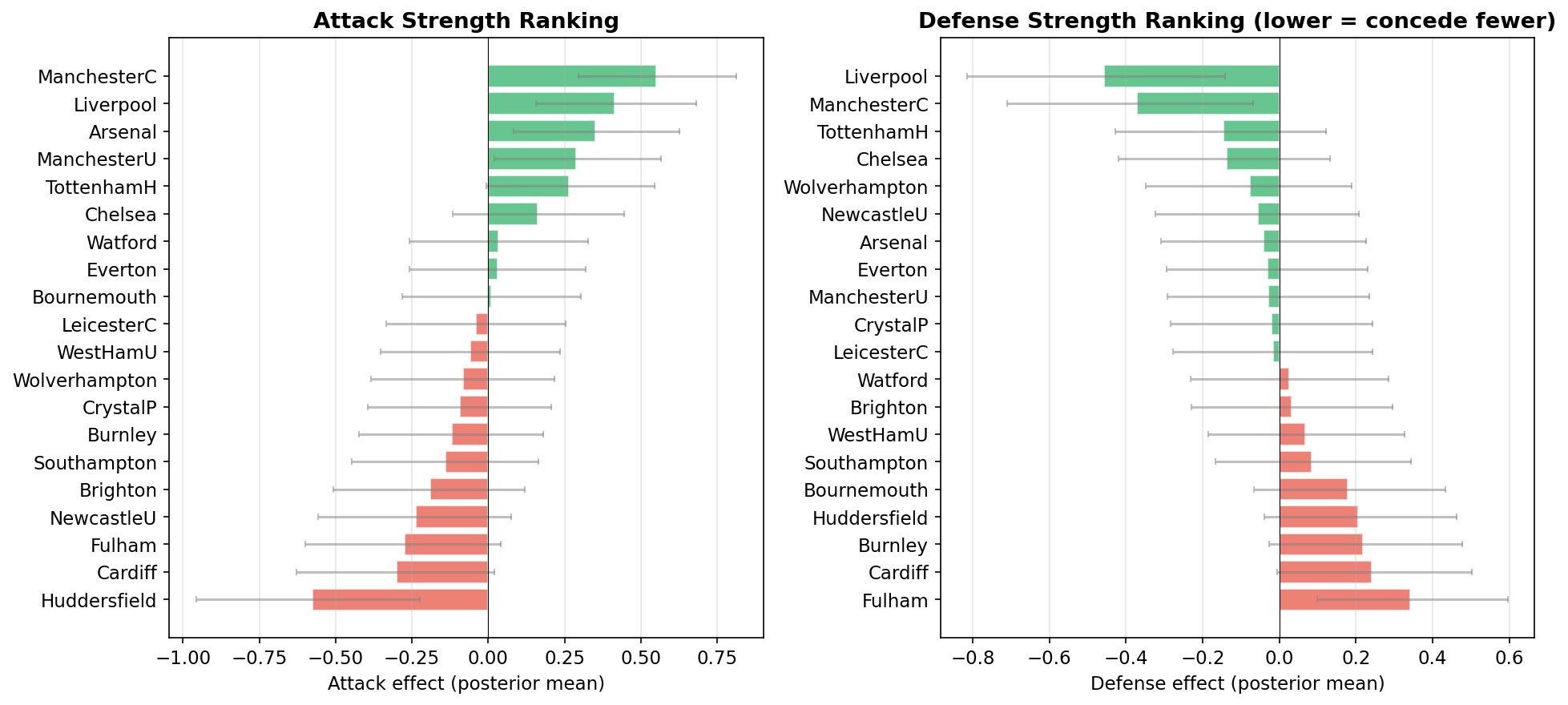
Home goal rate: 1.473Team Rankings
The attack and defense random effects provide a principled ranking of all 20 teams:
# Top 5 attack and defense
attack_means = result.summary_random['attack']['mean'].values[:20]
defense_means = result.summary_random['defense']['mean'].values[:20]

print("Top 5 Attack:")
for i in np.argsort(-attack_means)[:5]:
    print(f"  {id_to_team[i+1]:<16} {attack_means[i]:+.3f}")

print("\nTop 5 Defense (lowest = best):")
for i in np.argsort(defense_means)[:5]:
    print(f"  {id_to_team[i+1]:<16} {defense_means[i]:+.3f}")
Top 5 Attack:
ManchesterC +0.550
Liverpool +0.414
Arsenal +0.351
ManchesterU +0.289
TottenhamH +0.265
Top 5 Defense (lowest = best):
Liverpool -0.458
ManchesterC -0.372
TottenhamH -0.147
Chelsea -0.139
Wolverhampton -0.078Step 3: Simulate the Season
With the model fitted, we now use posterior predictive simulation to predict the final league table. The idea: draw parameter values from the posterior, replay every unplayed match using those parameters, and repeat 1,000 times to build a distribution over final standings.
3a. Draw Joint Posterior Samples
posterior_sample() draws samples from the joint posterior distribution of the full latent field. Each sample is a complete, correlated set of all model parameters: intercept, home effect, all 20 attack effects, and all 20 defense effects. Joint samples preserve correlations between parameters; sampling independently from marginals would lose this structure and underestimate prediction uncertainty.
import pyinla as pyinla_utils

n_sims = 1000
n_teams_sim = len(team_to_id)

# Separate played and unplayed matches
unplayed = matches_df[matches_df['home_goals'].isna()].copy()
played = matches_df[matches_df['home_goals'].notna()].copy()
print(f'Unplayed matches to simulate: {len(unplayed)}')

# Calculate current points from played matches
current_pts = {team: 0 for team in team_to_id.keys()}
for _, match in played.iterrows():
    hg, ag = int(match['home_goals']), int(match['away_goals'])
    ht, at = match['home_team'], match['away_team']
    if hg > ag:
        current_pts[ht] += 3
    elif hg < ag:
        current_pts[at] += 3
    else:
        current_pts[ht] += 1
        current_pts[at] += 1
Unplayed matches to simulate: 67Next, we draw 1,000 joint posterior samples and extract the individual parameter arrays. Each sample contains a latent vector (the full latent field concatenated) and _contents metadata that tells us where each component starts:
# Prepare arrays for posterior parameter samples
np.random.seed(42)
intercept_samples = np.zeros(n_sims)
home_samples = np.zeros(n_sims)
attack_samples = np.zeros((n_sims, n_teams_sim))
defense_samples = np.zeros((n_sims, n_teams_sim))

# Draw joint posterior samples from the fitted INLA model
samples = pyinla_utils.posterior_sample(n=n_sims, result=result, seed=42)
print(f'Generated {n_sims} joint posterior samples')

# The latent field is a single vector containing all parameters:
#   [intercept, home, attack_1, ..., attack_20, defense_1, ..., defense_20]
# The _contents metadata maps component names to their positions:
contents = samples[0].get('_contents', {})
tags = contents.get('tag', [])
starts = contents.get('start', [])
lengths = contents.get('length', [])

tag_info = {}
for tag, start, length in zip(tags, starts, lengths):
    tag_info[tag] = (start - 1, length)  # convert to 0-indexed

# Extract parameter positions
s_int, _ = tag_info['(Intercept)']
s_home, _ = tag_info['home']
s_att, l_att = tag_info['attack']
s_def, l_def = tag_info['defense']

# Slice each sample's latent vector into individual parameter arrays
for sim in range(n_sims):
    latent = np.asarray(samples[sim]['latent']).flatten()
    intercept_samples[sim] = latent[s_int]
    home_samples[sim] = latent[s_home]
    attack_samples[sim] = latent[s_att:s_att + l_att]
    defense_samples[sim] = latent[s_def:s_def + l_def]

print(f'Intercept: {intercept_samples.mean():.4f} +/- {intercept_samples.std():.4f}')
print(f'Home:      {home_samples.mean():.4f} +/- {home_samples.std():.4f}')
Generated 1000 joint posterior samples
Intercept: 0.1527 +/- 0.1040
Home: 0.2331 +/- 0.06933b. Simulate Each Unplayed Match
For each of the 1,000 posterior draws, we replay every unplayed match. The expected goals follow the same Poisson model used for fitting:
- Home team goals:
log(lambda) = intercept + home + attack[home_team] + defense[away_team] - Away team goals:
log(lambda) = intercept + attack[away_team] + defense[home_team]
The home team's expected goals include the home coefficient (home advantage), while the away team's do not. Each team's attack effect contributes to their own goals, and the opponent's defense effect determines how easy they are to score against.
# Simulate 1,000 complete seasons
np.random.seed(42)
final_points = np.zeros((n_sims, n_teams_sim))

for sim in range(n_sims):
    # Start with current points from matches already played
    sim_pts = np.array([current_pts[id_to_team[i+1]] for i in range(n_teams_sim)])

    # Simulate each unplayed match using this simulation's posterior parameters
    for _, match in unplayed.iterrows():
        ht_id = team_to_id[match['home_team']] - 1   # 0-indexed team IDs
        at_id = team_to_id[match['away_team']] - 1

        # Expected goals (log scale) from the Poisson GLMM
        log_lambda_home = (intercept_samples[sim] + home_samples[sim] +
                          attack_samples[sim, ht_id] + defense_samples[sim, at_id])
        log_lambda_away = (intercept_samples[sim] +
                          attack_samples[sim, at_id] + defense_samples[sim, ht_id])

        # Draw actual goals from Poisson distributions
        home_goals = np.random.poisson(np.exp(log_lambda_home))
        away_goals = np.random.poisson(np.exp(log_lambda_away))

        # Standard football points: 3 for win, 1 for draw, 0 for loss
        if home_goals > away_goals:
            sim_pts[ht_id] += 3
        elif away_goals > home_goals:
            sim_pts[at_id] += 3
        else:
            sim_pts[ht_id] += 1
            sim_pts[at_id] += 1

    final_points[sim] = sim_pts
Each simulation uses a different set of parameter values drawn from the posterior. This means parameter uncertainty (how confident the model is about each team's strength) propagates naturally into prediction uncertainty. A team with a well-estimated attack effect will have tighter prediction intervals than one with limited data.
3c. Aggregate into Probabilities
After simulating 1,000 complete seasons, we rank teams in each simulation and count how often each team finishes in the top 4 (Champions League qualification) or bottom 3 (relegation):
# Calculate top-4 and relegation probabilities
top4_probs = np.zeros(n_teams_sim)
relegation_probs = np.zeros(n_teams_sim)

for sim in range(n_sims):
    rankings = np.argsort(-final_points[sim])        # rank by points (descending)
    top4_probs[rankings[:4]] += 1                    # top 4 qualify for Champions League
    relegation_probs[rankings[-3:]] += 1             # bottom 3 are relegated

top4_probs /= n_sims       # fraction of simulations team finished in top 4
relegation_probs /= n_sims  # fraction of simulations team was relegated

print('Top-4 probabilities:')
for i in np.argsort(-top4_probs)[:6]:
    print(f'  {id_to_team[i+1]:<15} {top4_probs[i]*100:5.1f}%')

print('\nRelegation probabilities:')
for i in np.argsort(-relegation_probs)[:5]:
    print(f'  {id_to_team[i+1]:<15} {relegation_probs[i]*100:5.1f}%')
Top-4 probabilities:
ManchesterC 100.0%
Liverpool 100.0%
Arsenal 66.0%
TottenhamH 56.8%
ManchesterU 47.5%
Chelsea 29.7%
Relegation probabilities:
Huddersfield 100.0%
Fulham 100.0%
Cardiff 87.1%
Burnley 8.3%
Brighton 2.6%A 100% top-4 probability means the team finished in positions 1-4 in every simulation, not necessarily 1st place. Similarly, 100% relegation means the team finished in the bottom 3 (positions 18-20) in every simulation, not necessarily last. With 313 of 380 matches already played, there are 67 remaining matches to simulate, providing genuine uncertainty in the final standings for teams in the competitive mid-table zone.
We also compute expected points and 95% prediction intervals for each team:
# Summary statistics across all simulations
expected_pts = final_points.mean(axis=0)
pts_lower = np.percentile(final_points, 2.5, axis=0)
pts_upper = np.percentile(final_points, 97.5, axis=0)
Uncertainty propagates naturally through the full pipeline: posterior parameter uncertainty flows into match outcome uncertainty (via the Poisson draws), which flows into final standings uncertainty. This is the core advantage of simulation-based prediction over point estimates.
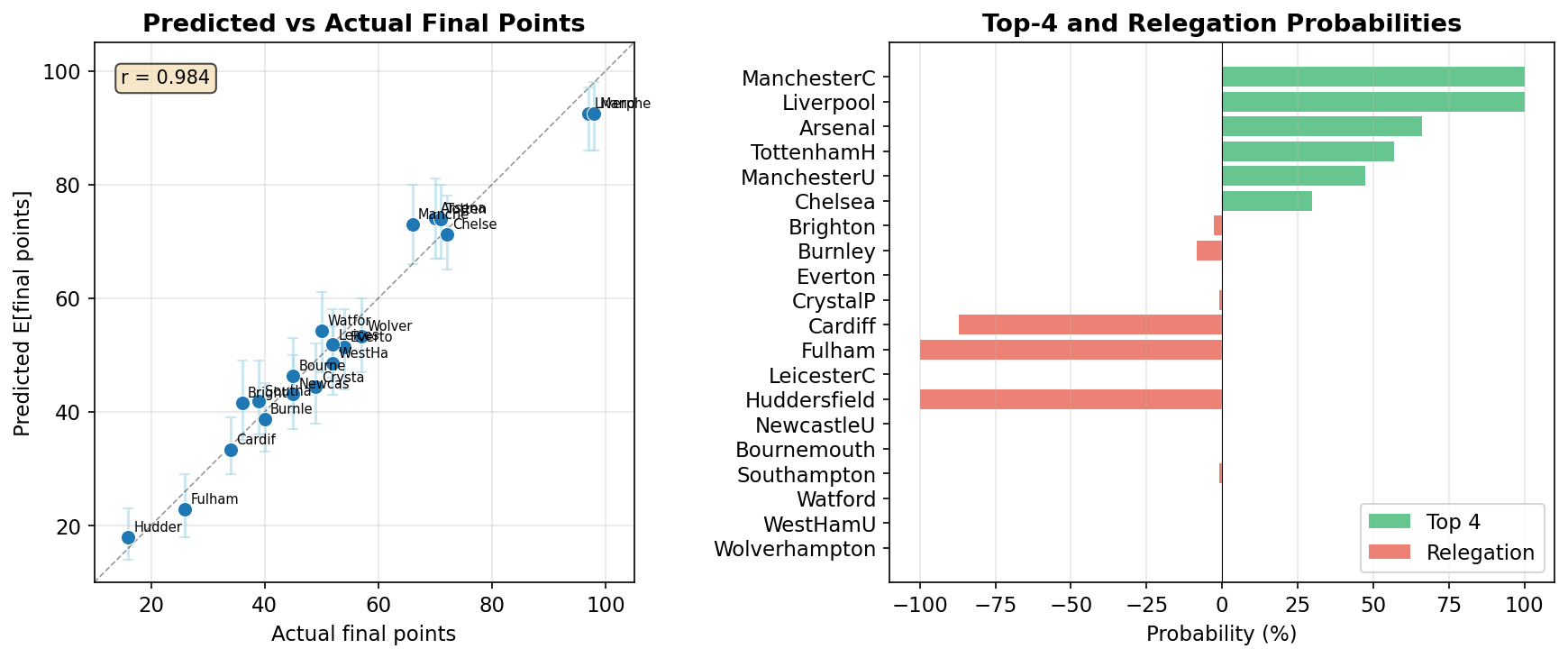
The model predictions correlate strongly with the actual final standings, demonstrating the practical value of Bayesian sports modeling for league table prediction.
Key Takeaways
- Poisson GLMMs with crossed random effects naturally model football match outcomes by separating team quality into attack and defense components.
- Home advantage is significant: playing at home increases expected goals by approximately 27%.
- pyINLA fits the model in about one second, making iterative modeling and real-time predictions practical.
- Posterior predictive simulation enables probabilistic league table predictions, including top-4 and relegation probabilities.
- Model-based predictions correlate well with actual outcomes, demonstrating the practical value of Bayesian sports modeling.
Going Further
This example demonstrates a straightforward Poisson GLMM, but football prediction can be extended in many directions. Some possibilities:
- Time-varying team strength: allow attack and defense effects to evolve over the season using random walk or autoregressive priors, capturing form changes and transfer window impacts.
- Player-level effects: incorporate individual player availability (injuries, suspensions) as covariates, since missing a key player can shift a team's expected performance.
- Score dependence: the basic Poisson model assumes home and away goals are independent. The Dixon-Coles correction or bivariate Poisson models can capture the tendency for low-scoring draws to occur more often than the independent model predicts.
- Overdispersion: replace the Poisson with a negative binomial likelihood to handle extra variability in goal counts.
- Additional covariates: rest days between matches, travel distance, derby effects, referee assignments, or weather conditions.
- Multi-season hierarchical models: share information across seasons by treating season-level team effects as draws from a higher-level distribution, enabling predictions for promoted teams with limited data.
- Tournament prediction: extend from league format to knockout tournaments (e.g., Champions League, World Cup) where elimination adds another layer of simulation.
Each extension adds complexity but also captures more of the rich structure in football data. pyINLA's speed makes it practical to iterate quickly through these modeling choices.
References
- Dixon, M.J. and Coles, S.G. (1997). "Modelling association football scores and inefficiencies in the football betting market." Journal of the Royal Statistical Society: Series C, 46(2), 265-280.
- Rue, H., Martino, S. and Chopin, N. (2009). "Approximate Bayesian inference for latent Gaussian models using integrated nested Laplace approximations." Journal of the Royal Statistical Society: Series B, 71(2), 319-392.