Skew Normal Distribution

Parametrization

The standardized Skew Normal distribution has the probability density function:

\[f(z) = \frac{2}{\omega_{\alpha}} \phi\left(\frac{z - \xi_{\alpha}}{\omega_{\alpha}}\right) \Phi\left(\alpha \frac{z - \xi_{\alpha}}{\omega_{\alpha}}\right)\]

where:

• \(\phi(\cdot)\) is the standard normal probability density function.

• \(\Phi(\cdot)\) is the standard normal cumulative distribution function.

• \(\omega_{\alpha}\) and \(\xi_{\alpha}\) are scale and location parameters reparameterized so that the mean is zero and variance is one.

• \(\alpha\) is the shape parameter controlling the asymmetry.

The Skew Normal likelihood is defined with respect to the response \(y_i\):

\[z_i = (y_i - \eta_i)\sqrt{w_i \tau} \sim f(z)\]

where:

• \(\pmb{y} = (y_1, y_2, \ldots, y_n)\) represents the observed continuous response values.

• \(\pmb{\eta} = (\eta_1, \eta_2, \ldots, \eta_n)\) is the linear predictor.

• \(\tau > 0\) is the precision parameter (inverse variance).

• \(w_i > 0\) is a fixed scale or weight (default \(w_i = 1\)).

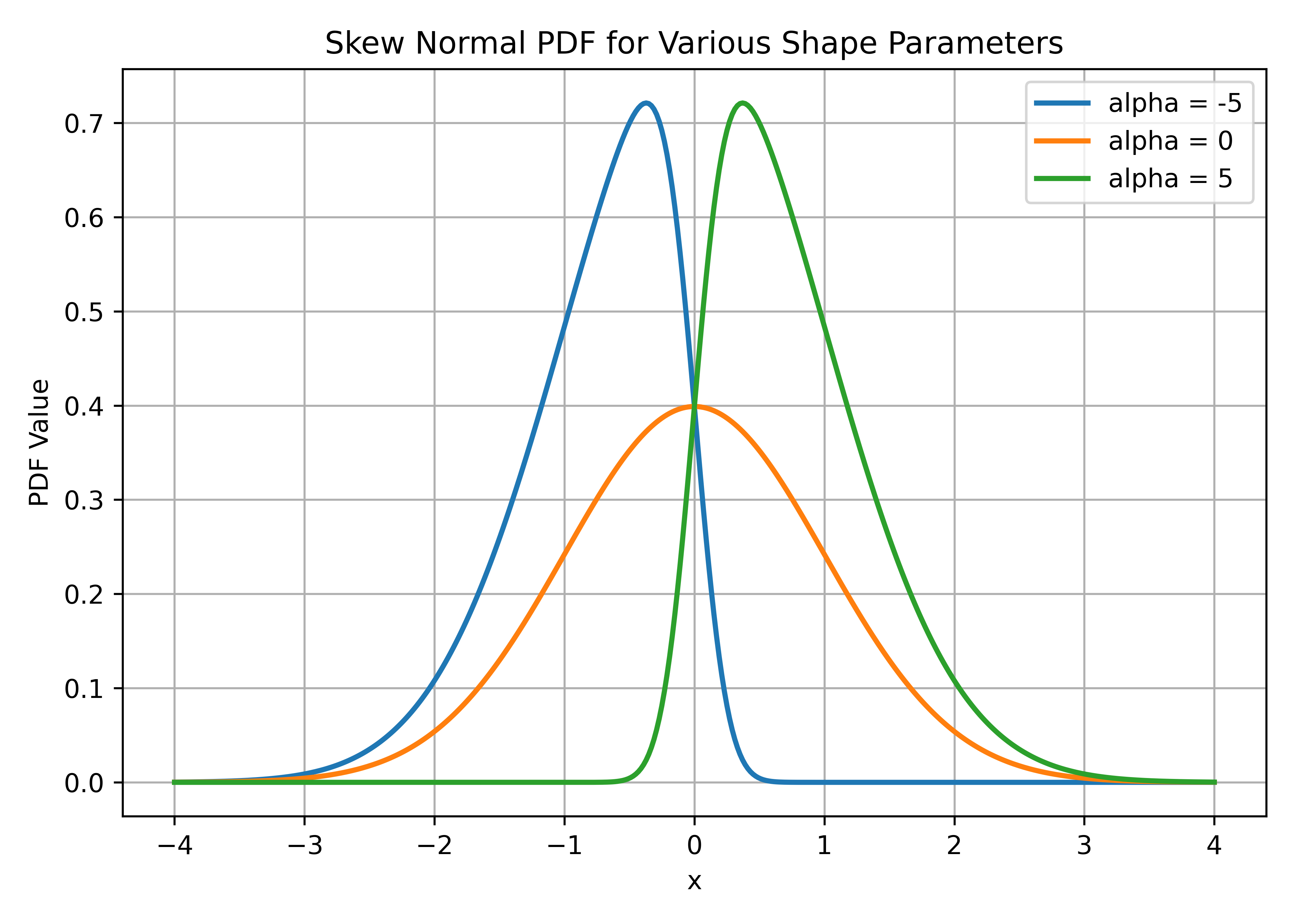
Figure 1 shows Skew Normal PDFs for different shape parameters. When \(\alpha = 0\), the distribution reduces to the standard Normal. Positive \(\alpha\) produces right skew, negative \(\alpha\) produces left skew.

Mean and Variance

For each observation \(y_i\):

\[\text{E}(y_i) = \eta_i, \quad \text{Var}(y_i) = \frac{1}{w_i \tau}\]

The mean equals the linear predictor (identity link), and the variance is controlled by the precision \(\tau\) and the observation-specific weight \(w_i\).

Link Function

The mean is linked to the linear predictor using the identity link (default):

\[\mu_i = \eta_i, \quad i = 1, 2, \ldots, n\]

In vector form:

\[\pmb{\mu} = \pmb{\eta}\]

Available link functions: default, identity.

Hyperparameters

The Skew Normal likelihood has two hyperparameters: precision \(\tau\) and skewness \(\gamma\). Both are represented internally via transformations to ensure they remain within valid ranges.

Hyperparameter \(\theta_1\) (precision)

Key: prec

The precision parameter \(\tau\) is represented internally as:

\[\theta_1 = \log(\tau)\]

Thus, \(\theta_1\) can take any real value, ensuring \(\tau > 0\). The prior is defined on \(\theta_1\). The default configuration uses a log-gamma prior with shape 1 and rate 5e-05, starting at \(\theta_1 = 4\) (corresponding to \(\tau \approx 54.6\)).

Hyperparameter \(\theta_2\) (skewness)

Key: skew

The standardized skewness \(\gamma\) is represented internally via a logit transformation:

\[\gamma = 0.988 \left(2 \frac{\exp(\theta_2)}{1 + \exp(\theta_2)} - 1\right)\]

This ensures \(|\gamma| < 0.988\). The standardized skewness relates to the shape parameter \(\alpha\) through:

\[\gamma = \frac{4-\pi}{2} \frac{\left(\delta \sqrt{2/\pi}\right)^3}{\left(1 - 2\delta^2/\pi\right)^{3/2}}, \quad \delta = \frac{\alpha}{\sqrt{1 + \alpha^2}}\]

The default configuration uses a PC prior (pc.sn) with parameter 10, which penalizes deviations from the base model (normal distribution with \(\gamma = 0\)).

When translated into control['family']['hyper'], the default entries look like:

control = {
    'family': {
        'hyper': [
            {
                'id': 'prec',
                'prior': 'loggamma',
                'param': [1, 5e-05],
                'initial': 4,
                'fixed': False,
            },
            {
                'id': 'skew',
                'prior': 'pc.sn',
                'param': [10],
                'initial': 0.00123456789,
                'fixed': False,
            },
        ]
    }
}

Each entry in control['family']['hyper'] may contain these keys:

• id - Hyperparameter identifier (prec or skew; positional aliases theta1 / theta2 also accepted).

• prior - Prior distribution name

• param - Prior parameters (list)

• initial - Initial value on the internal scale (log for prec, logit-bounded for skew)

• fixed - Whether to fix the hyperparameter (True/False)

Both hyperparameters accept any prior from the prior registry. The most commonly useful choices are:

Either hyperparameter can be pinned at a known value by setting fixed=True (no prior required). Unknown prior names raise a clear pyinla safety check: unknown prior '...' error before the engine runs; wrong param length similarly trips a safety error. Note that some prior/data combinations (e.g. flat on skew with small samples) may pass the safety layer but fail to converge in the INLA C engine.

Validation Rules

pyINLA enforces several validation rules for Skew Normal models to ensure correct specification:

Not Allowed Arguments

The following arguments are not allowed for skew normal and will raise PyINLAError:

• E (exposure) - Only allowed for poisson/nbinomial

• scale - Only allowed for gaussian/nbinomial/xbinomial/gamma/beta/logistic/t

• Ntrials - Only allowed for binomial/xbinomial/betabinomial/nbinomial2

• control['family']['variant'] - Not supported for skew normal

Hyperparameters

Key: control['family']['hyper']

When configuring hyperparameters (see the Hyperparameters section above for the full prior registry and key listing):

• If prior is omitted, the schema default is used (loggamma with param=[1, 5e-05] for prec; pc.sn with param=[10] for skew). A fixed entry can also omit prior and param.

• If specified, the prior name must be in the registry. Unknown names raise pyinla safety check: unknown prior.

• param length must match the prior's expected count.

Allowed Link Functions

Key: control['family']['link']

These link functions are supported:

• default

• identity

Specification

• family="sn"

• Required arguments:

  • \(\pmb{y}\): response vector of continuous values.

Notes

• When \(\gamma = 0\) (equivalently \(\alpha = 0\)), the skew normal reduces to the standard normal distribution.
• The standardized skewness \(\gamma\) is bounded: \(|\gamma| < 0.988\).
• Positive \(\gamma\) produces right (positive) skew; negative \(\gamma\) produces left (negative) skew.
• Data generation uses the reparameterization function to convert from moments \((\mu, \sigma^2, \gamma)\) to the \((\xi, \omega, \alpha)\) parameterization.

• Skew Normal Regression
• Skew Normal with Negative Skewness