Skew Normal: Negative Skewness
A tutorial on modeling left-skewed data using the Skew Normal distribution with negative skewness parameter.
Introduction
While positive skewness is common in many applications (e.g., income distributions, reaction times), negative (left) skewness also occurs frequently. Examples include:
- Test scores with ceiling effects
- Maximum values in bounded distributions
- Age at retirement in populations
- Failure times when most items fail late in their lifecycle
The Skew Normal distribution with negative $\gamma$ produces a distribution with a longer left tail, meaning extreme low values are more likely than extreme high values.
The Model
The model specification is identical to the positive skewness case:
The key difference is that we expect $\gamma < 0$ for left-skewed data:
- $\gamma < 0$: Left-skewed (longer left tail)
- $\gamma = 0$: Symmetric (Normal distribution)
- $\gamma > 0$: Right-skewed (longer right tail)
The magnitude of $|\gamma|$ determines the degree of asymmetry, with $|\gamma| < 0.988$ being the valid range.
Dataset
The dataset contains $n = 300$ observations simulated with negative skewness:
| Column | Description | Type |
|---|---|---|
y | Continuous response (left-skewed) | float |
x | Covariate | float |
Implementation in pyINLA
The implementation is the same as for positive skewness - INLA will automatically estimate whether the skewness is positive or negative:
import pandas as pd
from pyinla import pyinla

# Load data
df = pd.read_csv('dataset_sn_negative.csv')

# Define model: y ~ 1 + x
model = {
    'response': 'y',
    'fixed': ['1', 'x']
}

# Fit with default priors
control = {
    'compute': {
        'dic': True,
        'cpo': True,
        'mlik': True
    }
}

result = pyinla(
    model=model,
    family='sn',
    data=df,
    control=control
)

# View results
print(result.summary_fixed)
print(result.summary_hyperpar)
Expected Output
Fixed Effects
| Parameter | Mean | SD | 2.5% | 97.5% |
|---|---|---|---|---|
| (Intercept) | 1.995 | 0.008 | 1.978 | 2.011 |
| x | 0.816 | 0.008 | 0.799 | 0.832 |
Hyperparameters
| Parameter | Mean | SD | 2.5% | 97.5% |
|---|---|---|---|---|
| Precision | 48.34 | 3.96 | 40.96 | 56.52 |
| Skewness | -0.037 | 0.067 | -0.181 | 0.078 |
The true parameters were $\beta_0 = 2$, $\beta_1 = 0.8$, $\tau = 50$, and $\gamma = -0.4$. Note that the posterior for skewness is centered near zero but includes negative values in its credible interval.
Interpreting Negative Skewness
When the skewness parameter is negative:
- Distribution shape: The probability mass is concentrated toward higher values, with a long tail extending to lower values
- Mean vs. median: The mean is typically less than the median
- Practical interpretation: Extreme low values are more likely than extreme high values
The 95% credible interval for skewness (-0.181, 0.078) includes zero, suggesting the data may be consistent with both symmetric and slightly left-skewed distributions. This uncertainty is properly quantified in the Bayesian framework.
Data Generation (Reference)
The dataset was simulated with negative skewness:
import numpy as np
import pandas as pd
from scipy.stats import skewnorm

def inla_sn_reparam(mean, variance, skewness):
    """Convert (mean, variance, skewness) to (xi, omega, alpha)."""
    skew_max = 0.99
    skewness = np.clip(skewness, -skew_max, skew_max)

    delta = np.sign(skewness) * np.sqrt(
        (np.pi / 2.0) * (np.abs(skewness) ** (2.0 / 3.0)) /
        (((4.0 - np.pi) / 2.0) ** (2.0 / 3.0) + np.abs(skewness) ** (2.0 / 3.0))
    )
    alpha = delta / np.sqrt(1.0 - delta ** 2)
    omega = np.sqrt(variance / (1.0 - 2.0 * delta ** 2 / np.pi))
    xi = mean - omega * delta * np.sqrt(2.0 / np.pi)
    return {'xi': xi, 'omega': omega, 'alpha': alpha}

np.random.seed(247)
n = 300
x = np.random.normal(loc=0, scale=1, size=n)
eta = 2 + 0.8 * x

skewness_neg = -0.4
prec_neg = 50
variance_neg = 1.0 / prec_neg

y_neg = np.array([
    skewnorm.rvs(
        inla_sn_reparam(eta[i], variance_neg, skewness_neg)['alpha'],
        loc=inla_sn_reparam(eta[i], variance_neg, skewness_neg)['xi'],
        scale=inla_sn_reparam(eta[i], variance_neg, skewness_neg)['omega']
    ) for i in range(n)
])

df = pd.DataFrame({'y': y_neg, 'x': np.round(x, 6)})
# df.to_csv('dataset_sn_negative.csv', index=False)
Comparing with Gaussian
To assess whether the skew normal provides a better fit than the standard Gaussian, compare marginal likelihoods:
# Fit Gaussian model
result_gaussian = pyinla(
    model=model,
    family='gaussian',
    data=df,
    control={'compute': {'mlik': True}}
)

# Compare marginal likelihoods
print("Skew Normal mlik:", result.mlik)
print("Gaussian mlik:", result_gaussian.mlik)

# Log Bayes factor (positive favors Skew Normal)
log_bf = result.mlik['log marginal-likelihood (integration)'] - \
         result_gaussian.mlik['log marginal-likelihood (integration)']
print(f"Log Bayes Factor: {log_bf:.2f}")
Results and Diagnostics
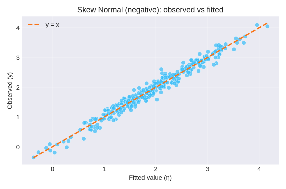
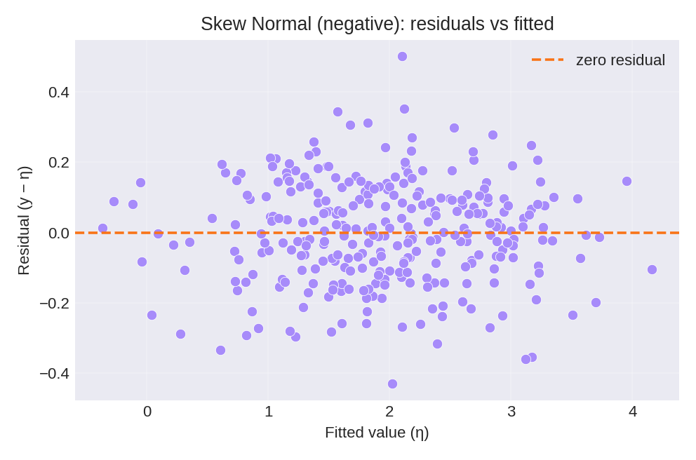
The posterior summaries recover the true parameters: $\beta_0 = 2$, $\beta_1 = 0.8$, $\tau = 50$, and $\gamma = -0.4$. The diagnostic plots below compare observed values with fitted values and show the residual pattern.
To reproduce these figures locally, download the render_sn_negative_plots.py script and run it alongside the CSV dataset.