Skew Normal Regression

Introduction

The Skew Normal distribution extends the Gaussian distribution by adding a shape parameter that captures asymmetry in the data. This is useful when the residuals or response distribution is not symmetric around the mean.

When the skewness parameter $\gamma = 0$, the Skew Normal reduces to the standard Normal distribution. Positive $\gamma$ produces right-skewed distributions (longer right tail), while negative $\gamma$ produces left-skewed distributions.

The Model

For each observation $i = 1, \ldots, n$, the response $y_i$ follows a Skew Normal distribution. The likelihood is defined via the standardized variable:

where the standardized Skew Normal PDF is:

with $\phi$ and $\Phi$ being the standard Normal PDF and CDF, and parameters $\xi_\alpha$, $\omega_\alpha$ chosen to ensure zero mean and unit variance.

The model parameters are:

• $y_i \in \mathbb{R}$ is the continuous response variable
• $\eta_i = \beta_0 + \beta_1 x_i$ is the linear predictor (location)
• $\tau > 0$ is the precision parameter
• $\gamma \in (-0.988, 0.988)$ is the skewness parameter
• $w_i > 0$ is an optional scale factor (default = 1)

Hyperparameters

The Skew Normal has two hyperparameters:

• Precision ($\tau$): Internal $\theta_1 = \log(\tau)$, default prior: loggamma(1, 5e-05)
• Skewness ($\gamma$): Internal representation via logit transformation, default prior: pc.sn(10)

The skewness is bounded: $|\gamma| < 0.988$. The PC prior on skewness penalizes deviation from the symmetric case ($\gamma = 0$).

Dataset

The dataset contains $n = 300$ observations with two columns:

• dataset_sn_regression.csv

Implementation in pyINLA

Fitting a Skew Normal regression model with custom prior on precision:

import pandas as pd
from pyinla import pyinla

# Load data
df = pd.read_csv('dataset_sn_regression.csv')

# Define model: y ~ 1 + x
model = {
    'response': 'y',
    'fixed': ['1', 'x']
}

# Use PC prior on precision (matching R-INLA documentation)
control = {
    'family': {
        'hyper': [
            {
                'id': 'prec',
                'prior': 'pc.prec',
                'param': [3, 0.01],
            },
        ]
    },
    'compute': {
        'dic': True,
        'cpo': True,
        'mlik': True
    }
}

# Fit the model
result = pyinla(
    model=model,
    family='sn',
    data=df,
    control=control
)

# View results
print(result.summary_fixed)
print(result.summary_hyperpar)

Extracting Results

The result object contains all posterior inference:

import numpy as np

# Fixed effects: posterior summaries for beta_0 and beta_1
print(result.summary_fixed)

# Extract posterior means
intercept = result.summary_fixed.loc['(Intercept)', 'mean']
slope = result.summary_fixed.loc['x', 'mean']

# Compute fitted values and residuals
x_vals = df['x'].to_numpy()
eta_hat = intercept + slope * x_vals
residuals = df['y'].to_numpy() - eta_hat

# Hyperparameters: precision and skewness
print(result.summary_hyperpar)

The summary_fixed DataFrame includes columns for mean, sd, 0.025quant, 0.5quant, 0.975quant, and mode.

Results and Diagnostics

The posterior summaries provide point estimates and credible intervals for $\beta_0$, $\beta_1$, precision $\tau$, and skewness $\gamma$.

The true parameters were $\beta_0 = 1$, $\beta_1 = 1$, $\tau = 100$, and $\gamma = 0.25$.

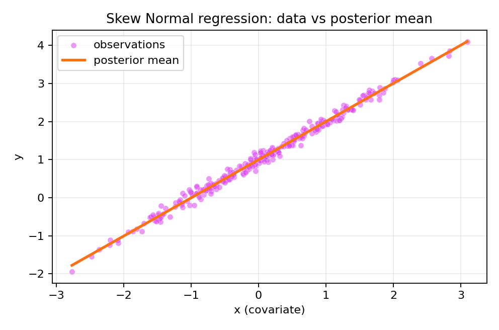
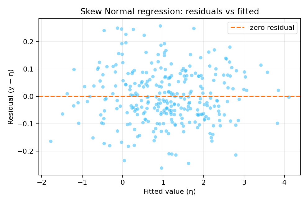
To reproduce these figures locally, download the render_skewnormal_plots.py script and run it alongside the CSV dataset.

Using Default Priors

For a simpler specification using default priors:

# Fit with default priors
control = {
    'compute': {
        'dic': True,
        'mlik': True
    }
}

result = pyinla(
    model=model,
    family='sn',
    data=df,
    control=control
)

print(result.summary_fixed)
print(result.summary_hyperpar)

The default priors are:

• prec: loggamma(1, 5e-05)
• skew: pc.sn(10)

Data Generation (Reference)

The dataset was simulated with the following parameters:

import numpy as np
import pandas as pd
from scipy.stats import skewnorm

def inla_sn_reparam(mean, variance, skewness):
    """Convert (mean, variance, skewness) to (xi, omega, alpha)."""
    skew_max = 0.99
    skewness = np.clip(skewness, -skew_max, skew_max)

    delta = np.sign(skewness) * np.sqrt(
        (np.pi / 2.0) * (np.abs(skewness) ** (2.0 / 3.0)) /
        (((4.0 - np.pi) / 2.0) ** (2.0 / 3.0) + np.abs(skewness) ** (2.0 / 3.0))
    )
    alpha = delta / np.sqrt(1.0 - delta ** 2)
    omega = np.sqrt(variance / (1.0 - 2.0 * delta ** 2 / np.pi))
    xi = mean - omega * delta * np.sqrt(2.0 / np.pi)
    return {'xi': xi, 'omega': omega, 'alpha': alpha}

np.random.seed(246)
n = 300
x = np.random.normal(loc=0, scale=1, size=n)
eta = 1 + x
skewness = 0.25
prec = 100
variance = 1.0 / prec

y = np.array([
    skewnorm.rvs(
        inla_sn_reparam(eta[i], variance, skewness)['alpha'],
        loc=inla_sn_reparam(eta[i], variance, skewness)['xi'],
        scale=inla_sn_reparam(eta[i], variance, skewness)['omega']
    ) for i in range(n)
])

df = pd.DataFrame({'y': y, 'x': np.round(x, 6)})
# df.to_csv('dataset_sn_regression.csv', index=False)