Parametrization
The Logistic distribution for a vector of observations \(\pmb{y} = (y_1, y_2, \ldots, y_n)\) has the following probability density function (PDF):
\[f(y_i \mid \mu_i, \tau, s) = \frac{\kappa \exp(-\kappa (y_i - \mu_i))}{(1 + \exp(-\kappa (y_i - \mu_i)))^{2}}, \quad i = 1, 2, \ldots, n\]
where:
\(\pmb{y} = (y_1, y_2, \ldots, y_n)\) represents the observed continuous response values.
\(\pmb{\mu} = (\mu_1, \mu_2, \ldots, \mu_n)\) represents the location parameters (mean) for each observation.
\(\kappa = \tau s \pi / \sqrt{3}\), where:
- \(\tau > 0\) is the precision parameter.
- \(s > 0\) is a fixed scaling factor (default = 1).
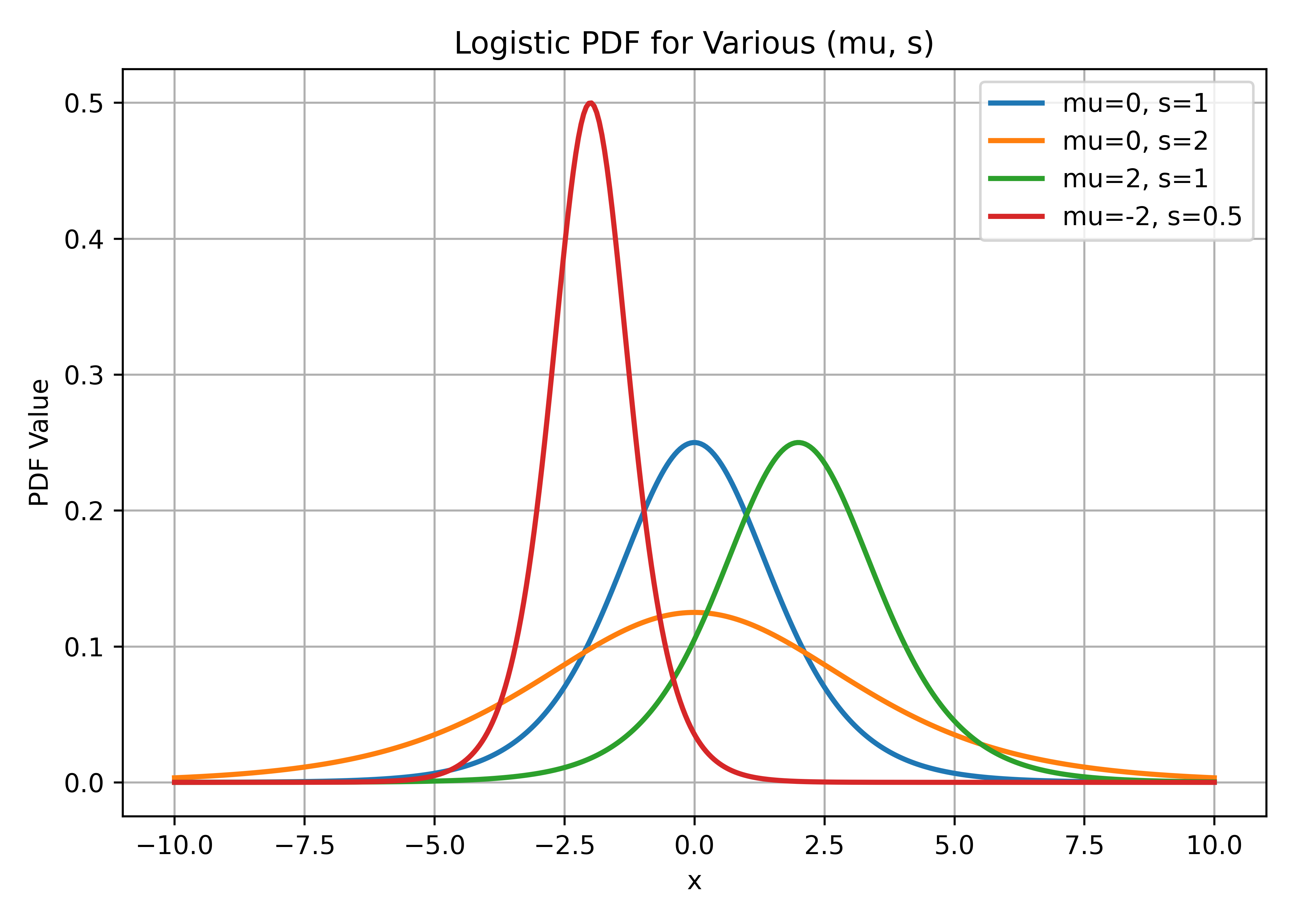
Figure 1 illustrates how the Logistic PDF changes for different location (\(\mu\)) and scale parameters.
Mean and Variance
The mean and variance of each observation \(y_i\) are given by:
\[\text{E}(y_i) = \mu_i, \quad \text{Var}(y_i) = \frac{1}{s \tau}\]
The variance is controlled by both the precision \(\tau\) and the fixed scaling factor \(s\). Higher precision or larger scale values result in smaller variance.
Link Function
The location parameter \(\mu_i\) is linked to the linear predictor \(\eta_i\) using the identity link (default):
\[\mu_i = \eta_i, \quad i = 1, 2, \ldots, n\]
In vector form:
\[\pmb{\mu} = \pmb{\eta}\]
Available link functions: default, identity.
Hyperparameters
The Logistic likelihood has one hyperparameter controlling the precision \(\tau\). This hyperparameter appears as a log-transformed parameter to ensure it remains within valid (positive) ranges and to improve numerical stability during inference.
Hyperparameter \(\theta\) (precision)
The default configuration assigns a loggamma prior to \(\theta\) with parameters \((1, 5\times 10^{-5})\). The initial value is set to \(\theta = 1\) (corresponding to \(\tau \approx 2.72\)).
Key: prec
The precision parameter \(\tau\) is represented internally as \(\theta = \log(\tau)\), so \(\theta\) can take any real value while ensuring \(\tau > 0\). The prior is defined on \(\theta\).
When translated into control['family']['hyper'], the default entry is:
control = {
    'family': {
        'hyper': [{
            'id': 'prec',
            'prior': 'loggamma',
            'param': [1, 5e-05],
            'initial': 1,
            'fixed': False,
        }]
    }
}
Each entry in control['family']['hyper'] may contain these keys:
id- Hyperparameter identifier (prec). Can be omitted for the first (and only) hyperparameter.prior- Prior distribution nameparam- Prior parameters (list)initial- Initial value on log scalefixed- Whether to fix the hyperparameter (True/False)
The precision hyperparameter (prec) accepts any prior from the prior registry. The most commonly useful choices on \(\theta = \log(\tau)\) are:
| Prior | Param shape | Use when |
|---|---|---|
loggamma (default) | [shape, rate], both positive | Conjugate prior on the log-precision; widely used. |
pc.prec | [U, alpha] with P(sd > U) = alpha | Penalised-complexity prior on the standard deviation. |
normal / gaussian | [mean, precision] on \(\theta\) | Soft Gaussian prior on the log-precision. |
flat | [] | Improper flat. Pass param=[] explicitly. |
logtnormal | [location, scale] | Truncated-normal on \(\theta\). |
The precision can also be pinned at a known value by setting fixed=True (no prior required). Unknown prior names raise a clear pyinla safety check: unknown prior '...' error before the engine runs; wrong param length similarly trips a safety error.
Validation Rules
pyINLA enforces several validation rules for Logistic models to ensure correct specification:
Not Allowed Arguments
The following arguments are not allowed for logistic and will raise PyINLAError:
E(exposure) - Only allowed for poisson/nbinomialNtrials- Only allowed for binomial/xbinomial/betabinomial/nbinomial2control['family']['variant']- Not supported for logistic
Scale
Key: scale
When providing the scale argument:
All values must be strictly positive (> 0)
Length must match the number of observations
Hyperparameters
Key: control['family']['hyper']
When configuring hyperparameters (see the Hyperparameters section above for the full prior registry and key listing):
If
prioris omitted, the schema default is used (loggammawithparam=[1, 5e-05]); a fixed entry can also omitpriorandparam.If specified, the prior name must be in the registry. Unknown names raise
pyinla safety check: unknown prior.paramlength must match the prior's expected count.
Allowed Link Functions
Key: control['family']['link']
These link functions are supported:
defaultidentity
Specification
family="logistic"- Required arguments:
- \(\pmb{y}\): response vector of continuous values
- \(\pmb{s}\): scale vector (keyword
scale, default = 1)
Basic Example
import numpy as np
import pandas as pd
from pyinla import pyinla

def rlogistic(n, mean=0, sd=1, rng=None):
    """Generate random samples from a logistic distribution."""
    if rng is None:
        rng = np.random.default_rng()
    p = rng.uniform(size=n)
    A = np.pi / np.sqrt(3)
    tauA = A / sd**2
    return (tauA * mean - np.log((1 - p) / p)) / tauA

# Simulate data
rng = np.random.default_rng(2026)
n = 1000
z = rng.normal(0, 0.1, size=n)
eta = 1 + z
y = rlogistic(n, mean=eta, sd=1, rng=rng)

data = pd.DataFrame({'y': y, 'z': z})

# Define the model
model = {'response': 'y', 'fixed': ['1', 'z']}

# Fit with logistic family
result = pyinla(
    model=model,
    family='logistic',
    data=data
)

print(result.summary_fixed)
print(result.summary_hyperpar)
Example with Scale Parameter
The scale parameter \(s\) allows for heteroscedastic models where variance differs across observations:
import pandas as pd
from pyinla import pyinla

# Load data with observation-specific scales
data = pd.read_csv('logistic_data.csv')

# Define the model
model = {'response': 'y', 'fixed': ['1', 'z']}

# Fit with scale parameter
result = pyinla(
    model=model,
    family='logistic',
    data=data,
    scale=data['scale'].to_numpy()
)

print(result.summary_fixed)
print(result.summary_hyperpar)
Notes
- The Logistic distribution has heavier tails than the Gaussian, making it more robust to outliers in the data.
- The scale parameter \(s\) can be observation-specific, enabling heteroscedastic modeling where variance varies across observations.
- When \(s = 1\) and \(\tau = 1\), the variance equals 1.