Logistic Regression: Observation Scale

Introduction

In many real-world applications, the variance of observations is not constant across all data points. This phenomenon, known as heteroscedasticity, can arise when measurement precision varies, when observations come from different sources, or when the variability naturally depends on some covariate.

The Logistic distribution in pyINLA supports observation-specific scale parameters $s_i$ that allow for heteroscedastic modeling. This tutorial demonstrates how to incorporate these scale factors into a regression model.

The Model

We extend the standard Logistic regression model by introducing observation-specific scale parameters. For each observation $i = 1, \ldots, n$:

where:

• $y_i \in \mathbb{R}$ is the continuous response variable
• $\mu_i = \eta_i = \beta_0 + \beta_1 z_i$ is the location parameter (linear predictor)
• $\tau > 0$ is the common precision parameter (estimated)
• $s_i > 0$ is the known scale factor for observation $i$ (fixed, not estimated)
• $\kappa_i$ is the observation-specific scale parameter in the Logistic PDF

The variance for each observation becomes:

Observations with larger $s_i$ have smaller variance (more precise), while observations with smaller $s_i$ have larger variance (less precise).

When to Use Scale Parameters

Observation-specific scale parameters are useful in several scenarios:

• Weighted regression: When some observations are more reliable than others (e.g., based on sample size or measurement precision)
• Meta-analysis: When combining results from multiple studies with different standard errors
• Grouped data: When observations represent group means with known within-group variances
• Heteroscedastic errors: When the error variance is known to vary systematically

The scale parameter effectively acts as a weight: larger values of $s_i$ give more weight to observation $i$ in the likelihood.

Dataset

The dataset contains $n = 500$ observations with three columns:

• dataset_logistic_scale.csv

Download the CSV file and place it in your working directory.

Implementation in pyINLA

To incorporate observation-specific scales, pass the scale vector to the scale argument of pyinla():

import pandas as pd
from pyinla import pyinla

# Load data with scale column
df = pd.read_csv('dataset_logistic_scale.csv')

# Define model: y ~ 1 + z
model = {
    'response': 'y',
    'fixed': ['1', 'z']
}

# Specify control options
control = {
    'compute': {
        'dic': True,
        'cpo': True,
        'mlik': True
    }
}

# Fit the model with observation-specific scales
result = pyinla(
    model=model,
    family='logistic',
    data=df,
    scale=df['scale'].to_numpy(),  # Pass scale vector
    control=control
)

# View posterior summaries
print(result.summary_fixed)
print(result.summary_hyperpar)

Important: The scale argument must be a numpy array (or array-like) with the same length as the number of observations. Each element $s_i$ should be positive.

Extracting Results

The results are extracted in the same way as for standard regression:

# Fixed effects: posterior summaries for regression coefficients
print(result.summary_fixed)

# Extract posterior means
intercept = result.summary_fixed.loc['(Intercept)', 'mean']
slope = result.summary_fixed.loc['z', 'mean']

# Hyperparameters: posterior summary for precision tau
# Note: The reported precision is the base precision,
# actual observation precision is tau * s_i
print(result.summary_hyperpar)

# Marginal likelihood for model comparison
print(result.mlik)

Results and Diagnostics

The posterior summaries provide estimates for $\beta_0$, $\beta_1$, and the base precision $\tau$. The true parameters used for data generation were $\beta_0 = 2$, $\beta_1 = 1.5$, and $\tau = 1$.

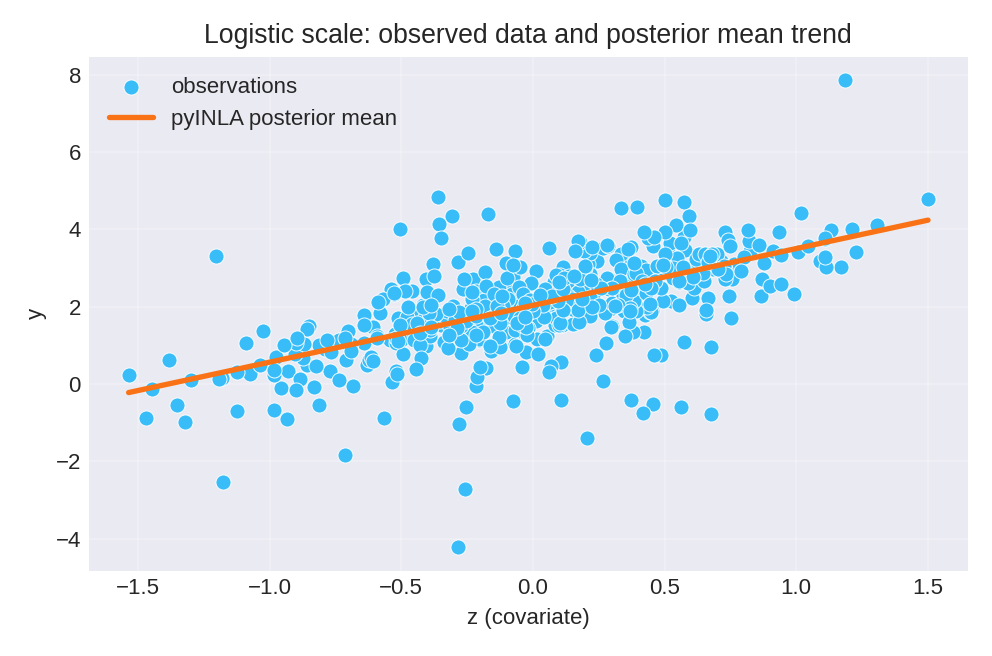
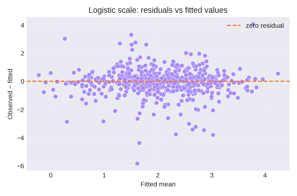
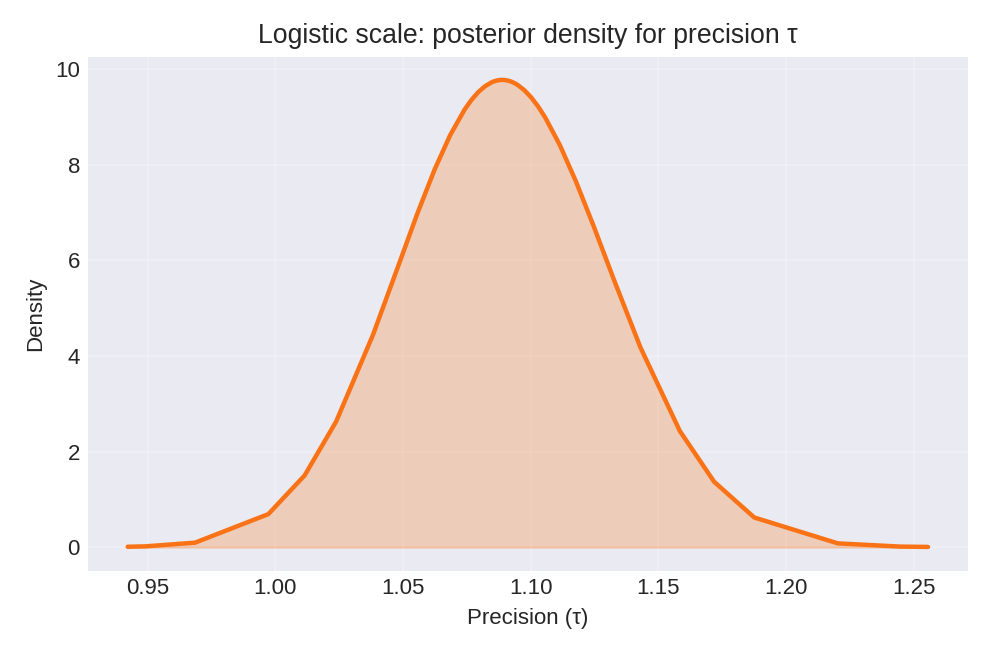
To reproduce these figures locally, download the render_logistic_plots.py script and run it alongside the CSV dataset.

Data Generation (Reference)

For reproducibility, the dataset was simulated with heteroscedastic errors:

with true parameter values: $\beta_0 = 2$, $\beta_1 = 1.5$, $\tau = 1$.

# Data generation script (for reference only)
import numpy as np
import pandas as pd

def rlogistic(n, mean=0, sd=1, rng=None):
    """Generate random samples from a logistic distribution."""
    if rng is None:
        rng = np.random.default_rng()
    p = rng.uniform(size=n)
    A = np.pi / np.sqrt(3)
    tauA = A / sd**2
    return (tauA * mean - np.log((1 - p) / p)) / tauA

rng = np.random.default_rng(2027)
n = 500

# Generate covariate
z = rng.normal(0, 0.5, size=n)

# Linear predictor
eta = 2 + 1.5 * z

# Generate heteroscedastic scales
scale = rng.uniform(0.5, 2.0, size=n)

# For logistic: variance = 1/(s*tau), so sd = 1/sqrt(s*tau)
# With tau=1 and varying s, sd = 1/sqrt(s)
y = np.array([
    rlogistic(1, mean=eta[i], sd=1/np.sqrt(scale[i]), rng=rng)[0]
    for i in range(n)
])

df = pd.DataFrame({
    'y': y,
    'z': np.round(z, 6),
    'scale': np.round(scale, 6)
})
# df.to_csv('dataset_logistic_scale.csv', index=False)

Interpretation Notes

• Scale vs. Weight: The scale parameter $s_i$ acts multiplicatively on the precision. Larger $s_i$ means smaller variance and effectively more "weight" for that observation.
• Reported Precision: The hyperparameter summary reports the base precision $\tau$. The effective precision for observation $i$ is $\tau \cdot s_i$.
• Standard Errors: By accounting for heteroscedasticity, the standard errors of the regression coefficients are more accurately estimated than in a homoscedastic model.
• Model Comparison: The DIC and marginal likelihood account for the scale structure, enabling fair comparison with alternative models.