Logistic Distribution Regression

Introduction

In this tutorial, we fit a Bayesian linear regression model where the response variable follows a Logistic distribution. The Logistic distribution is a continuous probability distribution with a symmetric, bell-shaped curve but heavier tails compared to the Gaussian distribution.

This makes the Logistic distribution particularly useful when modeling data that may contain outliers, as it provides a more robust alternative to normal errors while maintaining computational tractability.

The Model

We consider a linear regression model with $n$ observations. For each observation $i = 1, \ldots, n$, the response $y_i$ is modeled as:

y_i = \beta_0 + \beta_1 z_i + \varepsilon_i, \quad \varepsilon_i \stackrel{\text{iid}}{\sim} \text{Logistic}(0, \kappa^{-1})

where:

$y_i \in \mathbb{R}$ is the continuous response variable
$z_i \in \mathbb{R}$ is the covariate
$\beta_0$ is the intercept
$\beta_1$ is the slope coefficient
$\kappa = \tau s \pi / \sqrt{3}$ is the scale parameter, where $\tau > 0$ is the precision and $s > 0$ is a fixed scaling factor
$\varepsilon_i$ is the Logistic noise term

Linear Predictor

The linear predictor $\eta_i$ links the mean of the response to the covariates through a linear combination:

\eta_i = \beta_0 + \beta_1 z_i

For the Logistic likelihood with identity link, the location parameter equals the linear predictor:

\mathbb{E}[y_i \mid \eta_i] = \mu_i = \eta_i

In matrix notation, we can write $\boldsymbol{\eta} = \mathbf{X}\boldsymbol{\beta}$, where $\mathbf{X}$ is the design matrix with a column of ones (for the intercept) and a column containing the covariate values.

Likelihood Function

The probability density function for the Logistic distribution is:

f(y_i \mid \mu_i, \kappa) = \frac{\kappa \exp(-\kappa (y_i - \mu_i))}{(1 + \exp(-\kappa (y_i - \mu_i)))^{2}}

where $\kappa = \tau s \pi / \sqrt{3}$. The variance of each observation is:

\text{Var}(y_i) = \frac{1}{s \tau}

The likelihood for the full dataset $\mathbf{y} = (y_1, \ldots, y_n)^\top$ is the product of individual densities:

p(\mathbf{y} \mid \boldsymbol{\beta}, \tau) = \prod_{i=1}^{n} \frac{\kappa \exp(-\kappa (y_i - \eta_i))}{(1 + \exp(-\kappa (y_i - \eta_i)))^{2}}

Prior on the Precision

The precision parameter $\tau$ controls the spread of the distribution. In pyINLA, we work with the log-transformed precision $\theta = \log(\tau)$ to ensure positivity:

\theta = \log(\tau) \in \mathbb{R}

The default prior is a log-gamma distribution with parameters $a = 1$ and $b = 5 \times 10^{-5}$:

p(\theta) \propto \exp\bigl(a \cdot \theta - b \cdot e^{\theta}\bigr)

This corresponds to a Gamma$(a, b)$ prior on $\tau$ itself, which is vague enough to let the data inform the posterior while ensuring proper behavior.

Dataset

The dataset contains $n = 1000$ observations with two columns:

Column	Description	Type
`y`	Continuous response variable (Logistic distributed)	float
`z`	Covariate (predictor variable)	float

dataset_logistic.csv

Download the CSV file and place it in your working directory.

Implementation in pyINLA

We now fit the model using pyINLA. The key steps are:

Load the data into a pandas DataFrame
Define the model structure (response and fixed effects)
Specify the likelihood family as 'logistic'
Call the pyinla() function

import pandas as pd
from pyinla import pyinla

# Load data
df = pd.read_csv('dataset_logistic.csv')

# Define model: y ~ 1 + z (intercept + slope)
model = {
    'response': 'y',
    'fixed': ['1', 'z']
}

# Specify control options
control = {
    'compute': {
        'dic': True,
        'cpo': True,
        'mlik': True,
        'return_marginals': True
    }
}

# Fit the model with logistic family
result = pyinla(
    model=model,
    family='logistic',
    data=df,
    control=control
)

# View posterior summaries
print(result.summary_fixed)
print(result.summary_hyperpar)

Extracting Results

The result object contains all posterior inference. Here are the key attributes:

# Fixed effects: posterior summaries for beta_0 and beta_1
print(result.summary_fixed)

# Extract posterior means
intercept = result.summary_fixed.loc['(Intercept)', 'mean']
slope = result.summary_fixed.loc['z', 'mean']

# Hyperparameters: posterior summary for precision tau
print(result.summary_hyperpar)

# Access the marginal likelihood for model comparison
print(result.mlik)

The summary_fixed DataFrame includes columns for mean, sd, 0.025quant, 0.5quant, 0.975quant, and mode.

Results and Diagnostics

The posterior summaries provide estimates for $\beta_0$, $\beta_1$, and the precision $\tau$. The true parameters used for data generation were $\beta_0 = 1$, $\beta_1 = 1$, and $\tau = 1$.

Scatter plot of y versus z with fitted regression line — Observed data $(z_i, y_i)$ with the posterior mean regression line.

Residuals versus fitted values — Residuals $y_i - \hat{\eta}_i$ versus fitted values.

Posterior density for the estimated precision $\tau$.

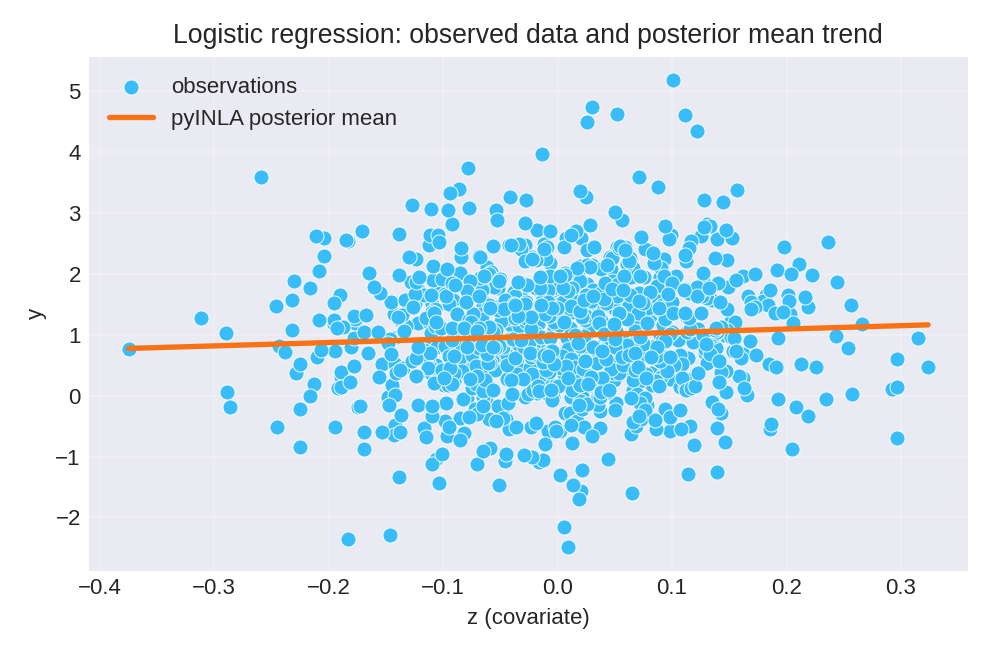
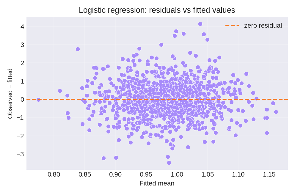
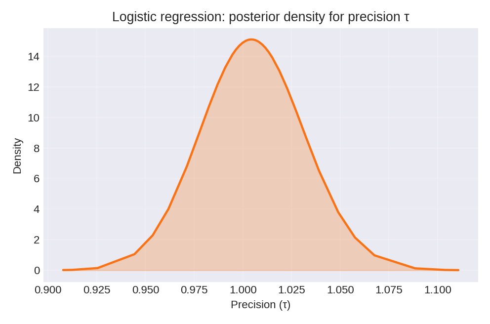
To reproduce these figures locally, download the render_logistic_plots.py script and run it alongside the CSV dataset.

Data Generation (Reference)

For reproducibility, the dataset was simulated from the following data-generating process:

z_i \stackrel{\text{iid}}{\sim} \mathcal{N}(0, 0.1), \quad \eta_i = \beta_0 + \beta_1 z_i, \quad y_i \sim \text{Logistic}(\eta_i, 1)

with true parameter values: $\beta_0 = 1$, $\beta_1 = 1$, $\tau = 1$ (i.e., $\sigma = 1$).

# Data generation script (for reference only)
import numpy as np
import pandas as pd

def rlogistic(n, mean=0, sd=1, rng=None):
    """Generate random samples from a logistic distribution."""
    if rng is None:
        rng = np.random.default_rng()
    p = rng.uniform(size=n)
    A = np.pi / np.sqrt(3)
    tauA = A / sd**2
    return (tauA * mean - np.log((1 - p) / p)) / tauA

rng = np.random.default_rng(2026)
n = 1000

# Generate covariate
z = rng.normal(0, 0.1, size=n)

# Linear predictor
eta = 1 + z

# Generate logistic response
y = rlogistic(n, mean=eta, sd=1, rng=rng)

df = pd.DataFrame({'y': y, 'z': np.round(z, 6)})
# df.to_csv('dataset_logistic.csv', index=False)