Log-Logistic Distribution

Parametrization

The Log-Logistic distribution for a random vector \(\pmb{y} = (y_1, y_2, \ldots, y_n)\), where each \(y_i > 0\), has two parameterization variants.

Variant 0 (default):

\[F_0(y_i) = \frac{1}{1 + \lambda_i y_i^{-\alpha}}, \quad y_i > 0\]

Variant 1:

\[F_1(y_i) = \frac{1}{1 + (\lambda_i y_i)^{-\alpha}}, \quad y_i > 0\]

where:

• \(\pmb{y} = (y_1, y_2, \ldots, y_n)\) represents the observed positive continuous response values.

• \(\alpha > 0\) is the shape parameter, controlling the tail behavior of the distribution.

• \(\lambda_i > 0\) is the scale parameter for observation \(y_i\), linked to the linear predictor.

The corresponding probability density functions (PDF) are:

Variant 0:

\[f_0(y_i) = \frac{\alpha \lambda_i y_i^{-\alpha - 1}}{(1 + \lambda_i y_i^{-\alpha})^2}, \quad y_i > 0\]

Variant 1:

\[f_1(y_i) = \frac{\alpha (\lambda_i y_i)^{-\alpha} \lambda_i}{(1 + (\lambda_i y_i)^{-\alpha})^2}, \quad y_i > 0\]

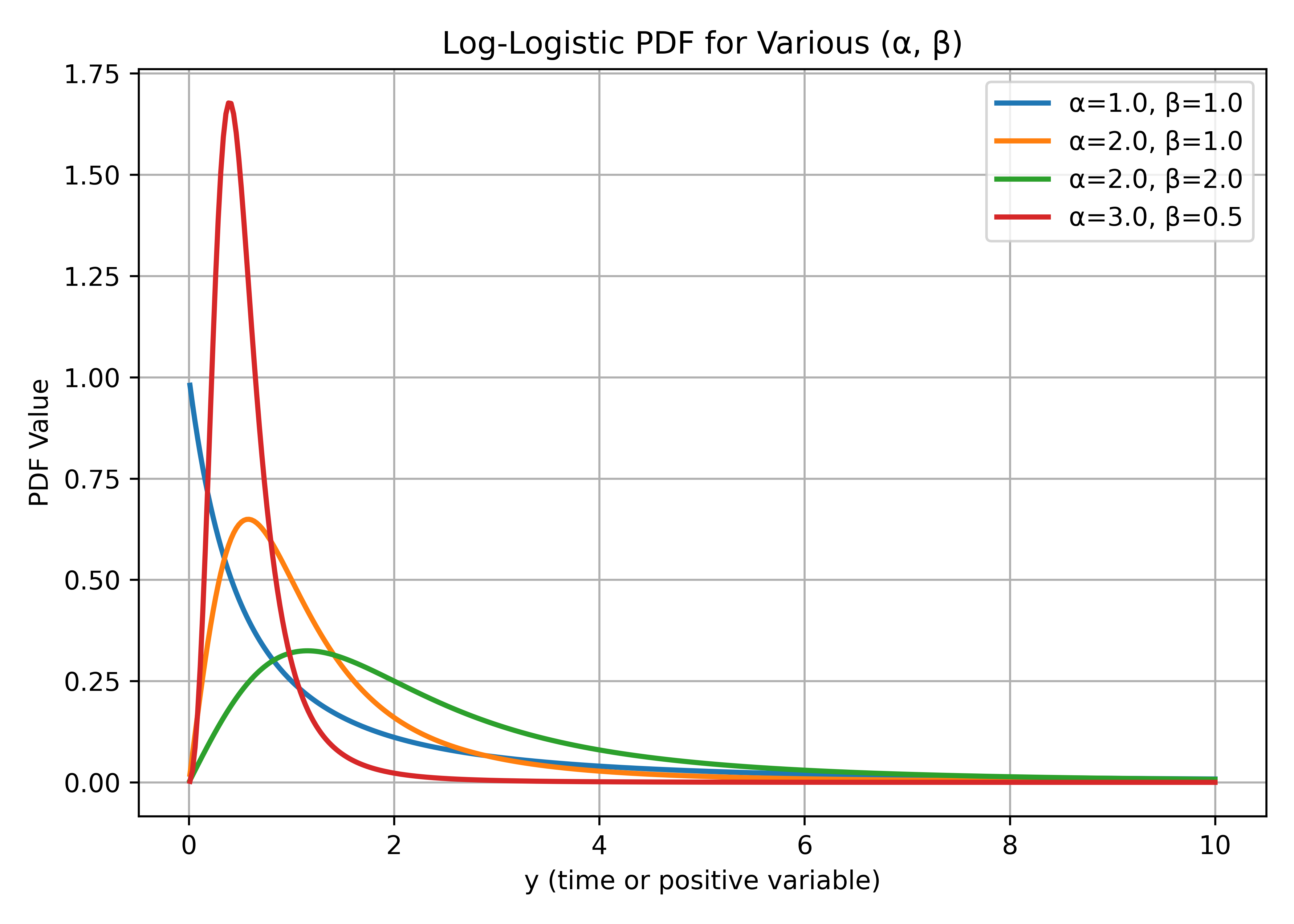
Figure 1 illustrates how the Log-Logistic PDF changes for different shape (\(\alpha\)) and scale parameters.

Mean and Variance

The mean and variance of \(y_i\) exist only for certain ranges of the shape parameter \(\alpha\):

• Mean: Exists if \(\alpha > 1\): \[\text{E}(y_i) = \lambda_i^{1/\alpha} \cdot \frac{\pi/\alpha}{\sin(\pi/\alpha)}\]

• Variance: Exists if \(\alpha > 2\) and involves higher-order moment expressions.

For small values of \(\alpha\), the distribution has very heavy tails and the moments may not exist.

Link Function

The scale parameter \(\lambda_i\) is linked to the linear predictor \(\eta_i\) using the log link (default):

\[\lambda_i = \exp(\eta_i), \quad i = 1, 2, \ldots, n\]

In vector form:

\[\pmb{\lambda} = \exp(\pmb{\eta})\]

Available link functions: default, log, neglog.

Hyperparameters

The Log-Logistic likelihood has one hyperparameter controlling the shape \(\alpha\). This hyperparameter appears as a log-transformed parameter to ensure it remains within valid (positive) ranges and to improve numerical stability during inference.

Hyperparameter \(\theta\) (shape)

The default configuration assigns a loggamma prior to \(\theta\) with parameters \((25, 25)\). The initial value is set to \(\theta = 1\) (corresponding to \(\alpha \approx 2.72\)).

Key: alpha

The shape parameter \(\alpha\) is represented internally as \(\theta = \log(\alpha)\), so \(\theta\) can take any real value while ensuring \(\alpha > 0\). The prior is defined on \(\theta\).

When translated into control['family']['hyper'], the default entry is:

control = {
    'family': {
        'variant': 0,  # or 1
        'hyper': [{
            'id': 'alpha',
            'prior': 'loggamma',
            'param': [25, 25],
            'initial': 1,
            'fixed': False,
        }]
    }
}

Each entry in control['family']['hyper'] may contain these keys:

• id - Hyperparameter identifier (alpha). Can be omitted for the first (and only) hyperparameter.

• prior - Prior distribution name

• param - Prior parameters (list)

• initial - Initial value on log scale

• fixed - Whether to fix the hyperparameter (True/False)

The shape hyperparameter (alpha) accepts any prior from the prior registry. The most commonly useful choices on \(\theta = \log(\alpha)\) are:

The shape can also be pinned at a known value by setting fixed=True (no prior required). Unknown prior names raise a clear pyinla safety check: unknown prior '...' error before the engine runs; wrong param length similarly trips a safety error.

Validation Rules

pyINLA enforces several validation rules for Log-Logistic models to ensure correct specification:

Not Allowed Arguments

The following arguments are not allowed for loglogistic and will raise PyINLAError:

• E (exposure) - Only allowed for poisson/nbinomial

• scale - Only allowed for gaussian/nbinomial/xbinomial/gamma/beta/logistic/t

• Ntrials - Only allowed for binomial/xbinomial/betabinomial/nbinomial2

Hyperparameters

Key: control['family']['hyper']

When configuring hyperparameters (see the Hyperparameters section above for the full prior registry and key listing):

• If prior is omitted, the schema default is used (loggamma with param=[25, 25]); a fixed entry can also omit prior and param.

• If specified, the prior name must be in the registry. Unknown names raise pyinla safety check: unknown prior.

• param length must match the prior's expected count.

Variant

Key: control['family']['variant']

The variant parameter is allowed and must be:

• 0 (default)

• 1

Allowed Link Functions

Key: control['family']['link']

For loglogistic:

• default

• log

• neglog

For loglogisticsurv:

• default

• log

• neglog

Response Values

Response variable \(\pmb{y}\) must be strictly positive (\(y_i > 0\)). pyINLA will raise PyINLAError if any response value is zero or negative.

Survival Response

When using loglogisticsurv, the response must be created using inla_surv():

from pyinla import inla_surv

# Create survival response (event=1 observed, event=0 right-censored)
y_surv = inla_surv(time=df["time"], event=df["event"])
result = pyinla(model={'response': y_surv, 'fixed': ['1', 'x']},
                family="loglogisticsurv", data=df)

inla_surv supports the following censoring types:

• Right censoring: the event has not occurred by the end of observation; only a lower bound on the survival time is known.
• Left censoring: the event occurred before observation began; only an upper bound is known.
• Interval censoring: the event is known to have occurred within a known time interval.

Survival-only Hyperparameters (cure model)

In addition to the shape alpha (which both forms share), loglogisticsurv exposes 10 cure-model regression coefficients beta1, ..., beta10 (positional aliases theta2, ..., theta11). The default priors are \(\text{Normal}(-4, 100)\) on beta1 (initial \(-5\)) and \(\text{Normal}(0, 100)\) on beta2, ..., beta10 (initial \(0\)). These are only active when a cure structure is configured; most survival users leave them at the defaults and configure only the alpha slot.

Specification

• family="loglogistic" for regression models

• family="loglogisticsurv" for survival models with censoring

• Required arguments:

  • For regression: \(\pmb{y}\) where \(y_i > 0\).

  • For survival: inla_surv(time, event) object.

• Optional: variant (0 or 1, default = 0).

Notes

• The Log-Logistic distribution has heavier tails than the log-normal, making it useful for modeling survival times with hazard rates that increase initially and then decrease.
• Two variant parameterizations are available (variant=0 or variant=1), choose the one that matches your data generation process.
• The survival model (loglogisticsurv) supports right censored, left censored, and interval censored data through the inla_surv object.
• If observed times are very large, consider scaling them to avoid numerical overflow issues.
• The hazard function of the log-logistic is non-monotonic when \(\alpha > 1\), first increasing and then decreasing.

• Log-Logistic Distribution Regression
• Log-Logistic Survival Analysis