Log-Logistic Survival Analysis
A tutorial on Bayesian survival analysis with the Log-Logistic distribution, supporting right-censored time-to-event data.
Introduction
The Log-Logistic distribution is popular in survival analysis because it:
- Has a closed-form survival function and hazard function
- Can model non-monotonic (unimodal) hazard rates
- Provides an alternative to log-normal when heavy tails are needed
- Is an accelerated failure time (AFT) model
This tutorial demonstrates using the loglogisticsurv family with censored data using the inla_surv response object.
The Model
For survival data, we observe $(t_i, \delta_i)$ for each subject $i$, where $t_i$ is the observed time and $\delta_i$ is the event indicator:
- $\delta_i = 1$: Event observed at time $t_i$
- $\delta_i = 0$: Right-censored at time $t_i$
The survival function for variant 0 is:
The hazard function is:
The hazard is:
- Monotonically decreasing when $\alpha \leq 1$
- Unimodal (rises then falls) when $\alpha > 1$
Dataset
The dataset contains $n = 1000$ observations with an event indicator:
| Column | Description | Type |
|---|---|---|
y | Observed time (event or censoring) | float |
x | Covariate (standardized) | float |
event | Event indicator (1=event, 0=censored) | int |
- dataset_loglogistic_surv_v0.csv (Variant 0)
- dataset_loglogistic_surv_v1.csv (Variant 1)
Implementation in pyINLA
For survival models, use inla_surv to create the response object:
import pandas as pd
from pyinla import pyinla, inla_surv

# Load data
df = pd.read_csv('dataset_loglogistic_surv_v0.csv')

# Create survival response object
y_surv = inla_surv(
    time=df['y'].to_numpy(),
    event=df['event'].to_numpy()
)

# Define model with survival response
model = {
    'response': y_surv,
    'fixed': ['1', 'x']
}

# Specify variant in control
control = {
    'family': {
        'variant': 0
    },
    'compute': {
        'dic': True,
        'cpo': True,
        'mlik': True
    }
}

# Fit the survival model
result = pyinla(
    model=model,
    family='loglogisticsurv',  # Note: 'surv' suffix
    data=df,
    control=control
)

# View results
print(result.summary_fixed)
print(result.summary_hyperpar)
Expected Output
Fixed Effects
| Parameter | Mean | SD | 2.5% | 97.5% |
|---|---|---|---|---|
| (Intercept) | 1.040 | 0.061 | 0.921 | 1.160 |
| x | 2.134 | 0.078 | 1.982 | 2.288 |
Hyperparameters
| Parameter | Mean | SD | 2.5% | 97.5% |
|---|---|---|---|---|
| alpha | 2.062 | 0.054 | 1.957 | 2.169 |
Note: With all events observed (no censoring), the survival model gives identical results to the regression model.
Results and Diagnostics
The posterior summaries recover the true parameters well. The fitted median $\hat{\lambda}^{1/\alpha}$ provides a natural summary for the log-logistic survival model.
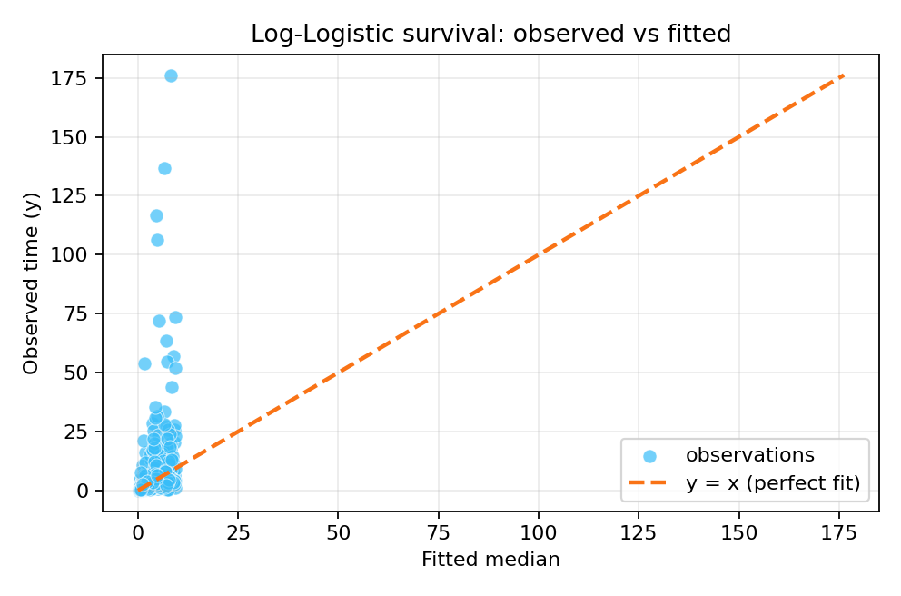
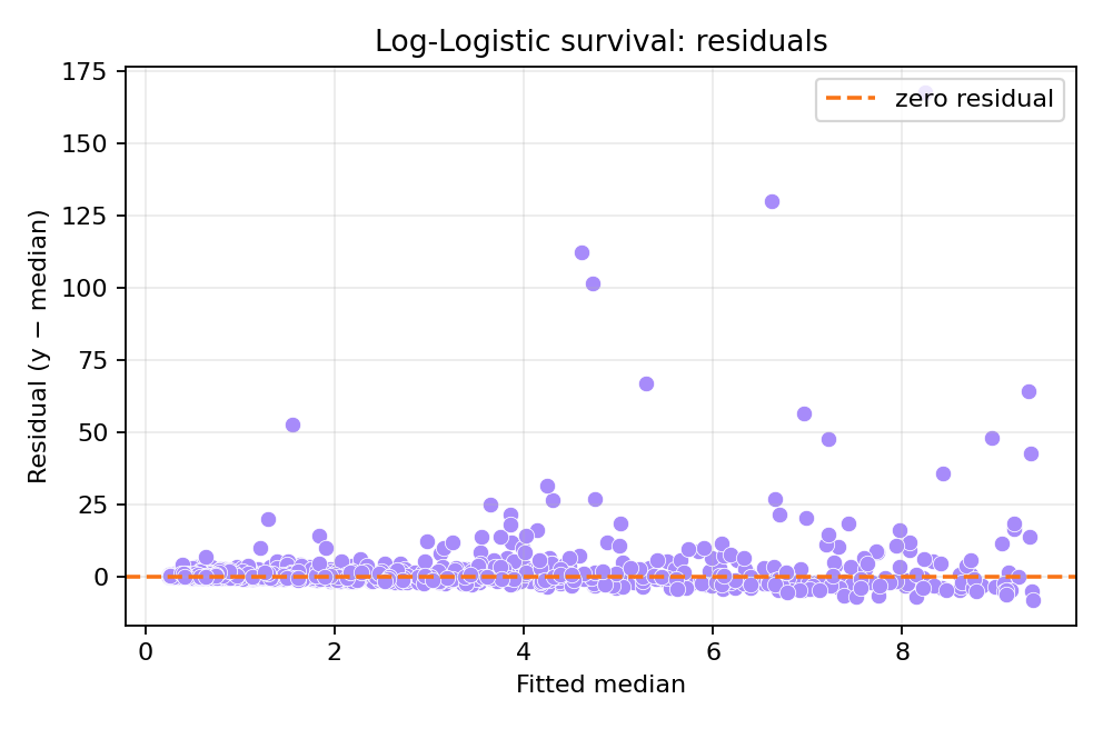
To reproduce these figures locally, download the render_loglogisticsurv_plots.py script and run it alongside the CSV dataset.
Using Variant 1
# Load data generated with variant 1
df_v1 = pd.read_csv('dataset_loglogistic_surv_v1.csv')

# Create survival response
y_surv_v1 = inla_surv(
    time=df_v1['y'].to_numpy(),
    event=df_v1['event'].to_numpy()
)

model_v1 = {
    'response': y_surv_v1,
    'fixed': ['1', 'x']
}

control_v1 = {
    'family': {
        'variant': 1
    },
    'compute': {
        'dic': True
    }
}

result_v1 = pyinla(
    model=model_v1,
    family='loglogisticsurv',
    data=df_v1,
    control=control_v1
)

print(result_v1.summary_fixed)
print(result_v1.summary_hyperpar)
Censoring Types
The inla_surv object supports various censoring types:
- Right censoring:
inla_surv(time, event)where event=0 means censored - Left censoring: Use
eventcolumn appropriately - Interval censoring: Provide interval bounds
# Example with mixed censoring
# For right-censored data: time is last observed, event=0
# For observed events: time is event time, event=1
# (`df['y']` holds the observed/censored time in the dataset used above.)

y_surv = inla_surv(
    time=df['y'].to_numpy(),
    event=df['event'].to_numpy()  # 1=event, 0=right-censored
)
Data Generation (Reference)
The survival dataset uses the same generation as the regression example, with an event indicator added:
import numpy as np
import pandas as pd

def rloglogistic(n, lam, alpha, variant=0, rng=None):
    """Generate random samples from a log-logistic distribution."""
    if rng is None:
        rng = np.random.default_rng()
    u = rng.uniform(size=n)
    if variant == 0:
        y = (lam / (1.0 / u - 1.0)) ** (1.0 / alpha)
    elif variant == 1:
        y = (1.0 / (1.0 / u - 1.0)) ** (1.0 / alpha) / lam
    return y

rng = np.random.default_rng(2026)
n = 1000
alpha = 2.1

# Generate covariate
x = rng.uniform(-1, 1, size=n)
x = (x - x.mean()) / x.std()

# Linear predictor
eta = 1.1 + 2.2 * x
lam = np.exp(eta)

# Generate log-logistic times
y = rloglogistic(n, lam=lam, alpha=alpha, variant=0, rng=rng)

# All events observed (no censoring in this example)
event = np.ones(n, dtype=int)

df = pd.DataFrame({
    'y': y,
    'x': np.round(x, 6),
    'event': event
})
# df.to_csv('dataset_loglogistic_surv_v0.csv', index=False)
Interpretation in AFT Framework
In the accelerated failure time (AFT) interpretation:
- Positive coefficients $\beta > 0$ indicate longer survival times
- The effect is multiplicative on the time scale
- Acceleration factor: $\exp(\beta)$ is the factor by which time is stretched/compressed
For example, with $\beta_1 = 2.134$:
- A one-unit increase in $x$ multiplies survival time by $\exp(2.134) \approx 8.45$
- Subjects with higher $x$ values survive substantially longer