Log-Logistic Regression
A tutorial on Bayesian regression with the Log-Logistic distribution for positive continuous data with heavy tails.
Introduction
The Log-Logistic distribution is a continuous probability distribution for positive values. It is commonly used in survival analysis and reliability engineering as an alternative to the log-normal and Weibull distributions. Key features include:
- Support on $(0, \infty)$
- Heavy tails suitable for modeling extreme values
- Closed-form CDF making it convenient for survival analysis
- Can exhibit non-monotonic hazard functions
The Model
For each observation $i = 1, \ldots, n$, the response $y_i > 0$ follows a Log-Logistic distribution. Two parameterization variants are available:
Variant 0 (default):
Variant 1:
where:
- $y_i > 0$ is the positive continuous response
- $\alpha > 0$ is the shape parameter (hyperparameter)
- $\lambda_i > 0$ is the scale parameter, linked via $\lambda_i = \exp(\eta_i)$
- $\eta_i = \beta_0 + \beta_1 x_i$ is the linear predictor
Hyperparameters
The Log-Logistic has one hyperparameter:
- Shape ($\alpha$): Internal $\theta = \log(\alpha)$, default prior: loggamma(1, 0.01)
The shape parameter controls the tail behavior:
- $\alpha < 1$: Monotonically decreasing hazard
- $\alpha = 1$: Monotonically decreasing hazard (special case)
- $\alpha > 1$: Unimodal (non-monotonic) hazard
Dataset
The dataset contains $n = 1000$ observations:
| Column | Description | Type |
|---|---|---|
y | Positive continuous response | float |
x | Covariate (standardized) | float |
- dataset_loglogistic_v0.csv (Variant 0)
- dataset_loglogistic_v1.csv (Variant 1)
Implementation in pyINLA
Fitting a Log-Logistic regression model with variant 0:
import pandas as pd
from pyinla import pyinla

# Load data (variant 0)
df = pd.read_csv('dataset_loglogistic_v0.csv')

# Define model: y ~ 1 + x
model = {
    'response': 'y',
    'fixed': ['1', 'x']
}

# Specify variant in control
control = {
    'family': {
        'variant': 0
    },
    'compute': {
        'dic': True,
        'cpo': True,
        'mlik': True
    }
}

# Fit the model
result = pyinla(
    model=model,
    family='loglogistic',
    data=df,
    control=control
)

# View results
print(result.summary_fixed)
print(result.summary_hyperpar)
Expected Output
Fixed Effects
| Parameter | Mean | SD | 2.5% | 97.5% |
|---|---|---|---|---|
| (Intercept) | 1.040 | 0.061 | 0.921 | 1.160 |
| x | 2.134 | 0.078 | 1.982 | 2.288 |
Hyperparameters
| Parameter | Mean | SD | 2.5% | 97.5% |
|---|---|---|---|---|
| alpha | 2.062 | 0.054 | 1.957 | 2.169 |
The true parameters were $\beta_0 = 1.1$, $\beta_1 = 2.2$, and $\alpha = 2.1$.
Results and Diagnostics
The posterior summaries recover the true parameters well. The fitted median $\hat{\lambda}^{1/\alpha}$ provides a natural summary for the log-logistic distribution.
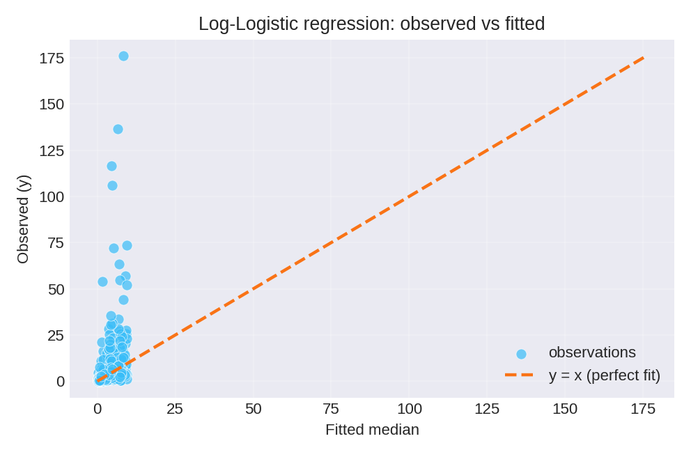
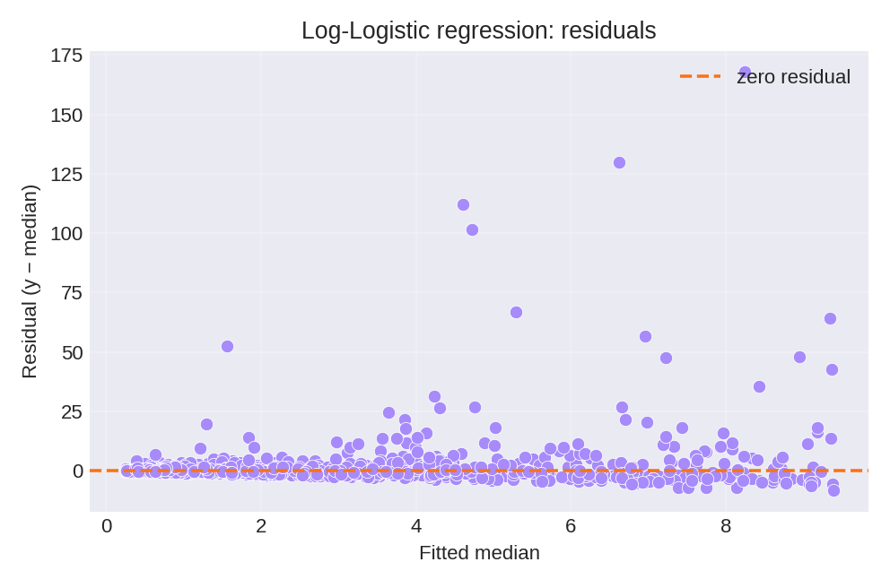
To reproduce these figures locally, download the render_loglogistic_plots.py script and run it alongside the CSV dataset.
Using Variant 1
For variant 1 parameterization:
# Load data generated with variant 1
df_v1 = pd.read_csv('dataset_loglogistic_v1.csv')

control_v1 = {
    'family': {
        'variant': 1
    },
    'compute': {
        'dic': True
    }
}

result_v1 = pyinla(
    model=model,
    family='loglogistic',
    data=df_v1,
    control=control_v1
)

print(result_v1.summary_fixed)
print(result_v1.summary_hyperpar)
The key difference between variants affects how the scale relates to $\lambda$:
- Variant 0: median = $\lambda^{1/\alpha}$
- Variant 1: median = $1/\lambda$
Data Generation (Reference)
The dataset was simulated with:
import numpy as np
import pandas as pd

def rloglogistic(n, lam, alpha, variant=0, rng=None):
    """Generate random samples from a log-logistic distribution."""
    if rng is None:
        rng = np.random.default_rng()
    u = rng.uniform(size=n)
    if variant == 0:
        y = (lam / (1.0 / u - 1.0)) ** (1.0 / alpha)
    elif variant == 1:
        y = (1.0 / (1.0 / u - 1.0)) ** (1.0 / alpha) / lam
    return y

rng = np.random.default_rng(2026)
n = 1000
alpha = 2.1

# Generate standardized covariate
x = rng.uniform(-1, 1, size=n)
x = (x - x.mean()) / x.std()

# Linear predictor and lambda
eta = 1.1 + 2.2 * x
lam = np.exp(eta)

# Generate log-logistic response (variant=0)
y = rloglogistic(n, lam=lam, alpha=alpha, variant=0, rng=rng)

df = pd.DataFrame({'y': y, 'x': np.round(x, 6)})
# df.to_csv('dataset_loglogistic_v0.csv', index=False)