Poisson Regression with Exposure Offset

Introduction

In this tutorial, we fit a Bayesian Poisson regression model for count data. The Poisson distribution is the natural choice for modeling non-negative integer outcomes such as the number of events occurring in a fixed period or region.

A key feature of Poisson regression is the exposure offset, which accounts for varying observation periods or population sizes across observations. This allows us to model rates rather than raw counts.

The Model

We consider a Poisson regression model with $n$ observations. For each observation $i = 1, \ldots, n$, the count response $y_i$ is modeled as:

y_i \sim \text{Poisson}(\lambda_i), \quad \lambda_i = E_i \cdot \exp(\eta_i)

where:

$y_i \in \{0, 1, 2, \ldots\}$ is the observed count
$\lambda_i > 0$ is the expected count (mean of the Poisson distribution)
$E_i > 0$ is the known exposure (offset) for observation $i$
$\eta_i$ is the linear predictor

The exposure $E_i$ allows the model to account for different observation periods, population sizes, or other scaling factors.

Linear Predictor

The linear predictor $\eta_i$ links the log-rate to the covariates through a linear combination:

\eta_i = \beta_0 + \beta_1 z_i

where $\beta_0$ is the intercept and $\beta_1$ is the slope coefficient for covariate $z_i$.

The Poisson distribution uses the log link function, so the expected count is:

\mathbb{E}[y_i \mid \eta_i, E_i] = \lambda_i = E_i \cdot \exp(\eta_i)

Equivalently, we can write:

\log(\lambda_i) = \log(E_i) + \eta_i

The term $\log(E_i)$ is called the offset in the linear predictor.

Likelihood Function

The probability mass function for a single observation is:

P(y_i \mid \lambda_i) = \frac{\lambda_i^{y_i} e^{-\lambda_i}}{y_i!}

The likelihood for the full dataset $\mathbf{y} = (y_1, \ldots, y_n)^\top$ is:

p(\mathbf{y} \mid \boldsymbol{\beta}, \mathbf{E}) = \prod_{i=1}^{n} \frac{\lambda_i^{y_i} e^{-\lambda_i}}{y_i!}

where $\lambda_i = E_i \cdot \exp(\beta_0 + \beta_1 z_i)$ and $\boldsymbol{\beta} = (\beta_0, \beta_1)^\top$.

Hyperparameters

The Poisson likelihood has no hyperparameters. Unlike the Gaussian distribution which has an unknown precision parameter, the Poisson distribution's variance equals its mean:

\text{Var}(y_i) = \mathbb{E}[y_i] = \lambda_i

This means there are no additional variance parameters to estimate. The model is fully determined by the regression coefficients $\boldsymbol{\beta}$.

Dataset

The dataset contains $n = 100$ observations with three columns:

Column	Description	Type
`y`	Count response variable	integer
`z`	Covariate (predictor variable)	float
`E`	Exposure offset	integer

dataset_poisson_regression.csv

Download the CSV file and place it in your working directory.

Implementation in pyINLA

We fit the model using pyINLA. The key steps are:

Load the data into a pandas DataFrame
Extract the exposure vector
Define the model structure (response and fixed effects)
Call pyinla() with family='poisson' and the exposure vector

import pandas as pd
from pyinla import pyinla

# Load data
df = pd.read_csv('dataset_poisson_regression.csv')
E = df['E'].to_numpy()

# Define model: y ~ 1 + z (intercept + slope)
model = {
    'response': 'y',
    'fixed': ['1', 'z']
}

# Fit the Poisson regression model with exposure offset
result = pyinla(
    model=model,
    family='poisson',
    data=df,
    E=E
)

# View posterior summaries for fixed effects
print(result.summary_fixed)

Extracting Results

The result object contains all posterior inference:

import numpy as np

# Fixed effects: posterior summaries for beta_0 and beta_1
print(result.summary_fixed)

# Extract posterior means
intercept = result.summary_fixed.loc['(Intercept)', 'mean']
slope = result.summary_fixed.loc['z', 'mean']

# Compute predicted rates (lambda_i = E_i * exp(eta_i))
eta_hat = intercept + slope * df['z'].to_numpy()
lambda_hat = df['E'].to_numpy() * np.exp(eta_hat)

# Compute residuals (observed - expected)
residuals = df['y'].to_numpy() - lambda_hat

The summary_fixed DataFrame includes columns for mean, sd, 0.025quant, 0.5quant, 0.975quant, and mode.

Results and Diagnostics

The posterior summaries provide estimates for $\beta_0$ and $\beta_1$. Since the Poisson likelihood has no hyperparameters, all inference concerns the fixed effects.

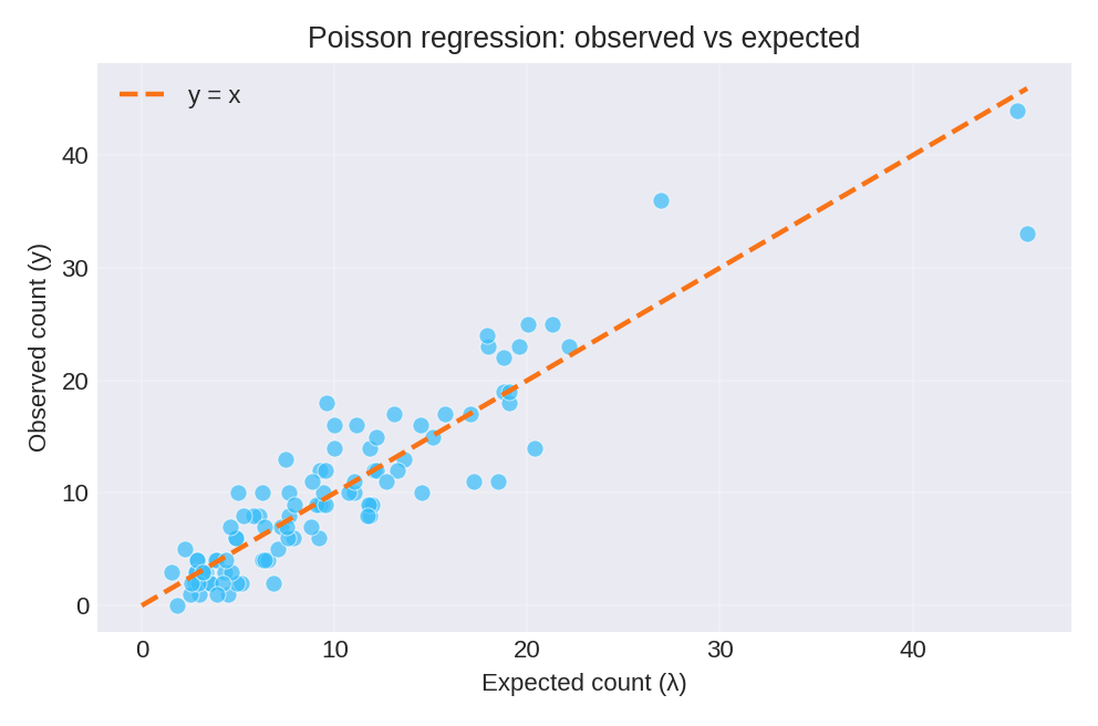
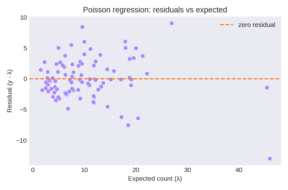
Observed counts versus expected counts with identity line — Observed counts $y_i$ versus expected counts $\hat{\lambda}_i = E_i \exp(\hat{\eta}_i)$.

Residuals versus expected counts — Residuals $y_i - \hat{\lambda}_i$ versus expected counts.

To reproduce these figures locally, download the render_poisson_plots.py script and run it alongside the CSV dataset.

Data Generation (Reference)

For reproducibility, the dataset was simulated from the following data-generating process:

z_i \stackrel{\text{iid}}{\sim} \mathcal{N}(0, 0.5^2), \quad E_i \sim \text{Uniform}\{2, 3, \ldots, 8\}, \quad y_i \sim \text{Poisson}(E_i \cdot \exp(\beta_0 + \beta_1 z_i))

with true parameter values: $\beta_0 = 0.5$, $\beta_1 = 1.0$.

# Data generation script (for reference only)
import numpy as np
import pandas as pd

rng = np.random.default_rng(2026)
n = 100
beta0, beta1 = 0.5, 1.0

z = rng.normal(scale=0.5, size=n)
E = rng.integers(2, 9, size=n)  # exposure between 2 and 8
eta = beta0 + beta1 * z
lambda_val = E * np.exp(eta)
y = rng.poisson(lam=lambda_val)

df = pd.DataFrame({'y': y, 'z': z, 'E': E})
# df.to_csv('dataset_poisson_regression.csv', index=False)