Gaussian Regression: Observation Scale

Introduction

In this tutorial, we fit a Bayesian linear regression model where each observation has its own variance scaling factor. This is useful when observations have different levels of reliability or when the variance is known to vary across the data.

The scale parameter in pyINLA allows us to specify observation-specific weights that modify the likelihood precision, enabling heteroskedastic modeling within the Gaussian framework.

The Model

We consider a linear regression model with $n$ observations where each observation $i$ has an associated scale factor $s_i > 0$. The response $y_i$ is modeled as:

where:

• $y_i \in \mathbb{R}$ is the continuous response variable
• $z_i \in \mathbb{R}$ is the covariate
• $\beta_0$ is the intercept
• $\beta_1$ is the slope coefficient
• $\tau > 0$ is the baseline observation precision
• $s_i > 0$ is the observation-specific scale factor
• $\varepsilon_i$ is the Gaussian noise term with observation-specific variance

The effective precision for observation $i$ is $\tau \cdot s_i$, so larger scale values correspond to more precise (lower variance) observations.

Linear Predictor

The linear predictor $\eta_i$ links the mean of the response to the covariates:

For the Gaussian likelihood with identity link, the mean of the response equals the linear predictor:

Note that the scale factors $s_i$ affect only the variance, not the mean structure.

Likelihood Function

Using the linear predictor and scale factors, the conditional distribution of $y_i$ is:

The likelihood for the full dataset $\mathbf{y} = (y_1, \ldots, y_n)^\top$ is:

where $\mathbf{s} = (s_1, \ldots, s_n)^\top$ is the vector of known scale factors.

Prior on the Precision

We place a log-gamma prior on the log-transformed baseline precision $\theta = \log(\tau)$:

This is equivalent to a Gamma$(a, b)$ prior on $\tau$:

Parameters used in this example: $a = 1.0$, $b = 0.01$, with initial value $\theta_0 = 2.0$.

Dataset

The dataset contains $n = 100$ observations with three columns:

• dataset_gaussian_main.csv

Download the CSV file and place it in your working directory.

Implementation in pyINLA

We fit the model using pyINLA by passing the scale vector to the scale parameter:

1. Load the data and extract the scale column
2. Define the model structure (response and fixed effects)
3. Specify the prior on the precision hyperparameter
4. Pass the scale vector to pyinla()

import pandas as pd
from pyinla import pyinla

# Load data
df = pd.read_csv('dataset_gaussian_main.csv')
scale_vec = df['scale'].to_numpy()

# Define model: y ~ 1 + z (intercept + slope)
model = {
    'response': 'y',
    'fixed': ['1', 'z']
}

# Specify log-gamma prior on precision: Gamma(a=1.0, b=0.01)
control = {
    'family': {
        'hyper': [{
            'prior': 'loggamma',
            'param': [1.0, 0.01],
            'initial': 2.0
        }]
    },
    'predictor': {'compute': True}  # enables fitted values
}

# Fit the model with observation-specific scale
result = pyinla(
    model=model,
    family='gaussian',
    data=df,
    scale=scale_vec,
    control=control
)

# View posterior summaries for fixed effects
print(result.summary_fixed)

Extracting Results

The result object contains all posterior inference:

# Fixed effects: posterior summaries for beta_0 and beta_1
print(result.summary_fixed)

# Extract posterior means
intercept = result.summary_fixed.loc['(Intercept)', 'mean']
slope = result.summary_fixed.loc['z', 'mean']

# Fitted values: posterior mean of eta_i
fitted_means = result.summary_fitted_values['mean'].to_numpy()

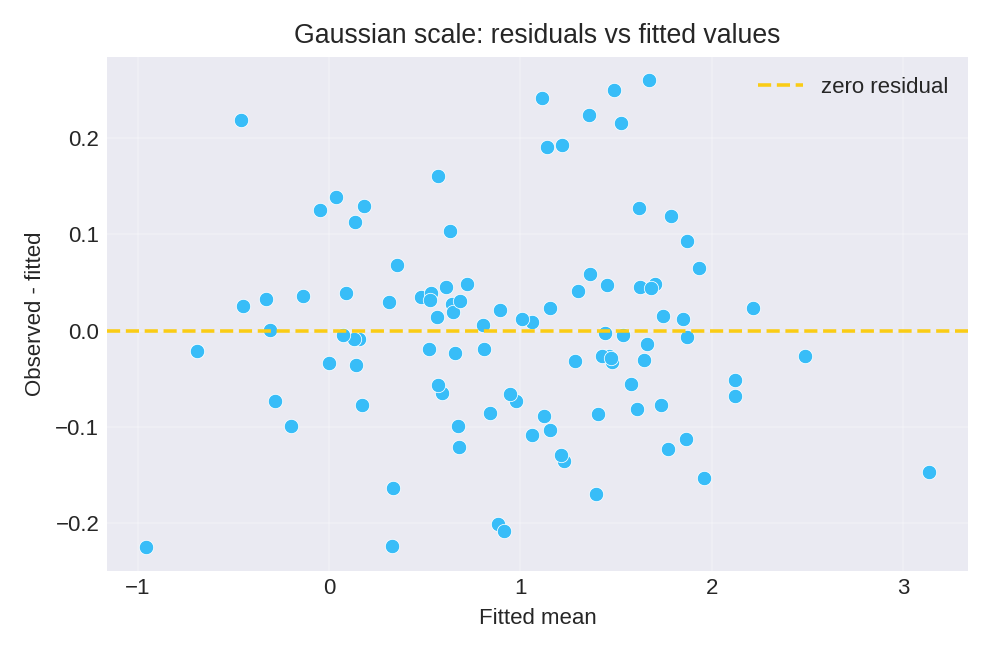
# Compute residuals
residuals = df['y'].to_numpy() - fitted_means

# Hyperparameters: posterior summary for baseline precision tau
print(result.summary_hyperpar)

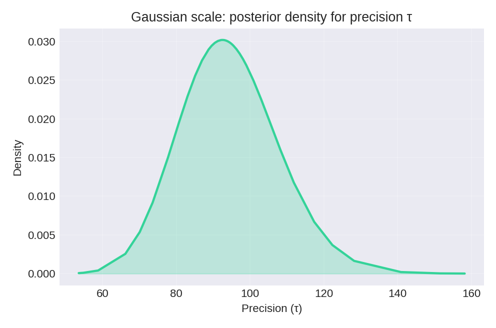
# Marginal posterior density for tau (for plotting)
density = result.marginals_hyperpar['Precision for the Gaussian observations']

The summary_fixed DataFrame includes columns for mean, sd, 0.025quant, 0.5quant, 0.975quant, and mode.

Results and Diagnostics

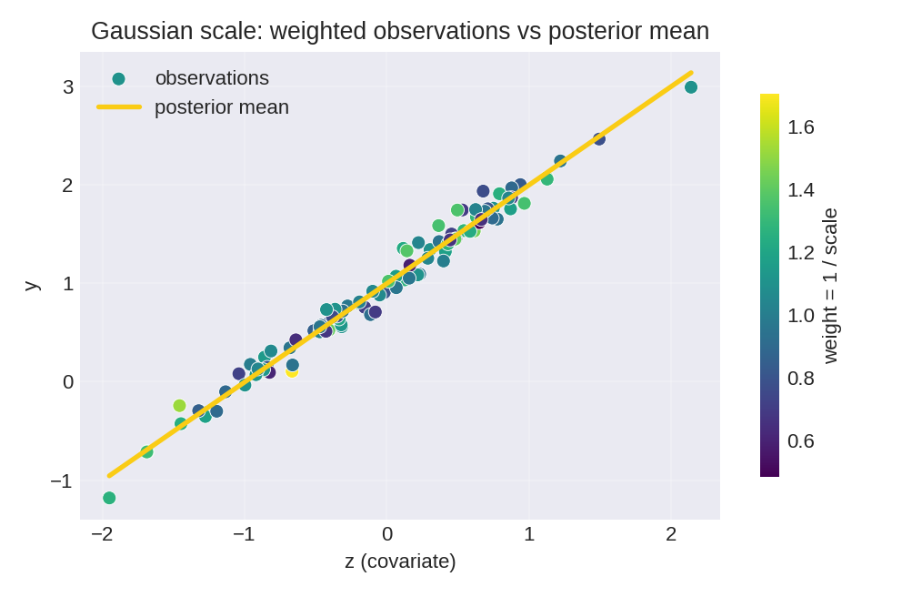
The posterior summaries provide point estimates and credible intervals for $\beta_0$, $\beta_1$, and the baseline precision $\tau$.

To reproduce these figures locally, download the render_gaussian_plots.py script and run it alongside the CSV dataset.

Recovered Parameters

The posterior means closely recover the true parameter values ($\beta_0 = 1$, $\beta_1 = 1$):

print(result.summary_fixed)

                 mean        sd  0.025quant  0.5quant  0.975quant      mode
(Intercept)  1.008805  0.007360    0.994342  1.008805    1.023267  1.008805
z            1.008208  0.007665    0.993147  1.008208    1.023269  1.008208

Both coefficients have posterior means within 1% of the true values, with narrow 95% credible intervals that contain the true values.

Data Generation (Reference)

For reproducibility, the dataset was simulated from the following data-generating process:

with true parameter values: $\beta_0 = 1$, $\beta_1 = 1$, $\tau = 100$.

# Data generation script (for reference only)
import numpy as np
import pandas as pd

rng = np.random.default_rng(42)
n = 100
beta0, beta1 = 1.0, 1.0
tau = 100.0  # baseline precision

z = rng.normal(size=n)
s = rng.lognormal(mean=0.0, sigma=0.25, size=n)  # scale factors
epsilon = rng.normal(scale=1.0/np.sqrt(tau * s), size=n)
y = beta0 + beta1 * z + epsilon

df = pd.DataFrame({'y': y, 'z': z, 'scale': s})
# df.to_csv('dataset_gaussian_main.csv', index=False)