Gaussian Regression: Precision Offset

Introduction

In this tutorial, we fit a Bayesian linear regression model where part of the observation variance is known a priori. This is common when measurements have a known instrument error or when combining data sources with different reliability levels.

The precision offset in pyINLA allows us to fix a known variance component while still estimating the remaining unknown variance from the data.

The Model

We consider a linear regression model where the total observation variance is the sum of two components:

y_i = \beta_0 + \beta_1 x_i + \varepsilon_i, \quad \varepsilon_i \stackrel{\text{iid}}{\sim} \mathcal{N}\left(0, \sigma^2_{\text{total}}\right)

where the total variance decomposes as:

\sigma^2_{\text{total}} = \sigma^2_0 + \sigma^2_1 = \frac{1}{\tau_0} + \frac{1}{\tau_1}

Here:

$\sigma^2_0 = 1/\tau_0$ is the known variance component (e.g., measurement error)
$\sigma^2_1 = 1/\tau_1$ is the unknown variance to be estimated
$\tau_0$ is the precision offset (fixed)
$\tau_1$ is the precision parameter (estimated)

Linear Predictor

The linear predictor $\eta_i$ links the mean of the response to the covariates:

\eta_i = \beta_0 + \beta_1 x_i

For the Gaussian likelihood with identity link:

\mathbb{E}[y_i \mid \eta_i] = \mu_i = \eta_i

Likelihood Function

The effective precision of each observation combines both components. In pyINLA's parameterization:

\tau_{\text{eff}} = \frac{1}{1/\tau_1 + 1/\tau_0} = \frac{\tau_0 \tau_1}{\tau_0 + \tau_1}

The likelihood for observation $y_i$ is:

y_i \mid \eta_i, \tau_1, \tau_0 \sim \mathcal{N}\left(\eta_i, \tau_{\text{eff}}^{-1}\right)

When $\tau_0$ is fixed at a known value, only $\tau_1$ is estimated from the data.

The Precision Offset

The precision offset $\tau_0$ is specified on the log scale as $\theta_0 = \log(\tau_0)$. Given a known variance $\sigma^2_0$, we compute:

\theta_0 = \log(\tau_0) = \log\left(\frac{1}{\sigma^2_0}\right) = -\log(\sigma^2_0)

Example: For a known variance of $\sigma^2_0 = 1.0$:

\theta_0 = \log(1/1.0) = \log(1) = 0

This value is passed to pyINLA via 'id': 'precoffset' with 'fixed': True.

Dataset

The dataset contains $n = 100$ observations with two columns:

Column	Description	Type
`y`	Continuous response variable	float
`x`	Covariate (predictor variable)	float

dataset_gaussian_offset.csv

Download the CSV file and place it in your working directory.

Implementation in pyINLA

We fit the model by specifying the precision offset as a fixed hyperparameter:

Define the known variance component $\sigma^2_0$
Convert to log precision: $\theta_0 = \log(1/\sigma^2_0)$
Pass to control['family']['hyper'] with 'id': 'precoffset'
Set 'fixed': True to keep it constant

import math
import pandas as pd
from pyinla import pyinla

# Load data
df = pd.read_csv('dataset_gaussian_offset.csv')

# Known variance component
var0 = 1.0  # known measurement variance

# Define model: y ~ 1 + x (intercept + slope)
model = {
    'response': 'y',
    'fixed': ['1', 'x']
}

# Specify the precision offset (fixed)
control = {
    'family': {
        'hyper': [{
            'id': 'precoffset',
            'initial': math.log(1.0 / var0),  # log(tau_0) = log(1/var0)
            'fixed': True
        }]
    },
    'predictor': {'compute': True}  # enables fitted values
}

# Fit the model
result = pyinla(
    model=model,
    family='gaussian',
    data=df,
    control=control
)

# View posterior summaries for fixed effects
print(result.summary_fixed)

Extracting Results

The result object contains posterior inference for the estimated parameters:

# Fixed effects: posterior summaries for beta_0 and beta_1
print(result.summary_fixed)

# Extract posterior means
intercept = result.summary_fixed.loc['(Intercept)', 'mean']
slope = result.summary_fixed.loc['x', 'mean']

# Fitted values: posterior mean of eta_i
fitted_means = result.summary_fitted_values['mean'].to_numpy()

# Compute residuals
residuals = df['y'].to_numpy() - fitted_means

# Hyperparameters: posterior summary for estimated precision tau_1
print(result.summary_hyperpar)

# Marginal posterior density for tau_1 (for plotting)
density = result.marginals_hyperpar['Precision for the Gaussian observations']

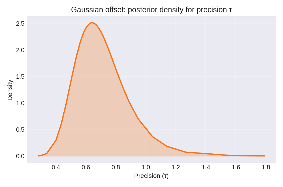
Note: The precision offset $\tau_0$ is fixed, so only $\tau_1$ appears in the hyperparameter summaries.

Results and Diagnostics

The posterior summaries provide estimates for $\beta_0$, $\beta_1$, and the unknown precision $\tau_1$.

Scatter plot of y versus x with fitted regression line — Observed data $(x_i, y_i)$ with the posterior mean regression line.

Residuals versus fitted values — Residuals $y_i - \hat{\eta}_i$ versus fitted values.

Posterior density for the estimated precision $\tau_1$.

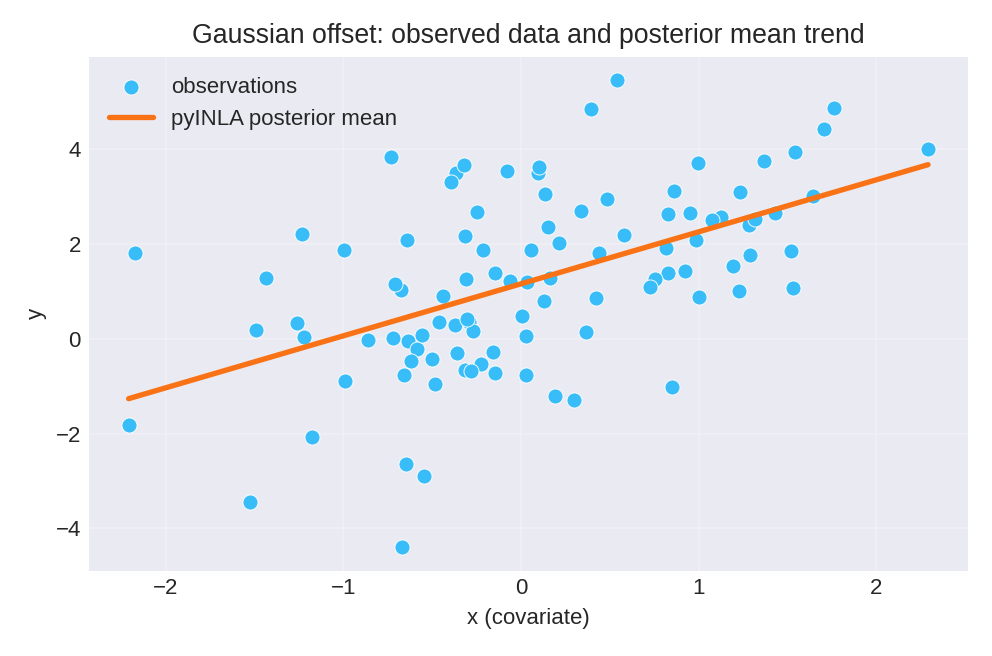
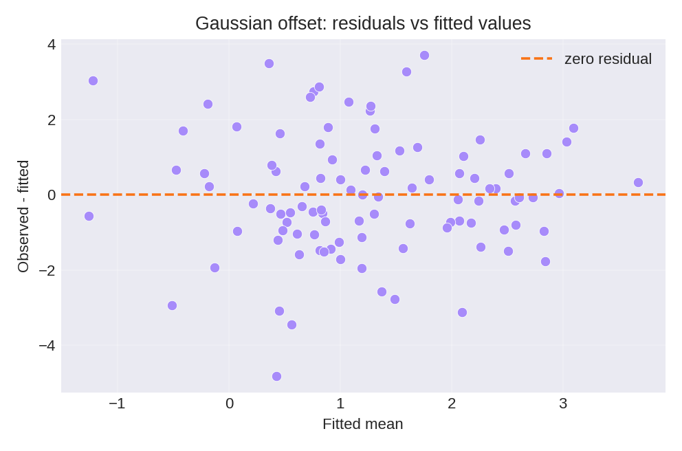
To reproduce these figures locally, download the render_gaussian_plots.py script and run it alongside the CSV dataset.

Data Generation (Reference)

For reproducibility, the dataset was simulated from the following data-generating process:

x_i \stackrel{\text{iid}}{\sim} \mathcal{N}(0, 1), \quad y_i = \beta_0 + \beta_1 x_i + \varepsilon_i, \quad \varepsilon_i \stackrel{\text{iid}}{\sim} \mathcal{N}(0, \sigma^2_0 + \sigma^2_1)

with true parameter values: $\beta_0 = 1$, $\beta_1 = 1$, $\sigma^2_0 = 1.0$ (known), $\sigma^2_1 = 2.0$ (to be estimated).

# Data generation script (for reference only)
import numpy as np
import pandas as pd

rng = np.random.default_rng(123)
n = 100
beta0, beta1 = 1.0, 1.0
var0 = 1.0  # known (fixed) variance component
var1 = 2.0  # unknown variance component (to be estimated)

x = rng.normal(size=n)
total_sd = np.sqrt(var0 + var1)  # sqrt(3.0) ≈ 1.73
epsilon = rng.normal(scale=total_sd, size=n)
y = beta0 + beta1 * x + epsilon

df = pd.DataFrame({'y': y, 'x': x})
# df.to_csv('dataset_gaussian_offset.csv', index=False)