Beta-Binomial Regression

Introduction

In this tutorial, we fit a Bayesian Beta-Binomial regression model for count data arising from repeated Bernoulli trials with overdispersion. The Beta-Binomial distribution is the natural choice when the probability of success varies across observations, leading to extra-binomial variation.

Unlike the standard Binomial distribution (where success probability is fixed), the Beta-Binomial has an overdispersion parameter that captures heterogeneity in success probabilities across observations.

The Model

We consider a Beta-Binomial regression model with $n$ observations. For each observation $i = 1, \ldots, n$, the count response $y_i$ follows a hierarchical model:

p_i \sim \text{Beta}(\alpha_i, \beta_i), \qquad y_i \mid p_i \sim \text{Binomial}(N_i, p_i)

Marginalizing over $p_i$, the response follows a Beta-Binomial distribution:

\pi(y_i) = \binom{N_i}{y_i} \frac{B(y_i + \alpha, N_i - y_i + \beta)}{B(\alpha, \beta)}, \quad y_i = 0, 1, \ldots, N_i

where $B(\cdot, \cdot)$ is the Beta function and $N_i$ is the number of trials for observation $i$.

Mean and Variance

The mean and variance of each observation are:

\mu_i = N_i \mu_p, \qquad \sigma_i^2 = N_i \mu_p (1 - \mu_p) \left(1 + (N_i - 1) \rho\right)

where:

$\mu_p = \frac{\alpha}{\alpha + \beta}$ is the mean probability from the Beta distribution
$\rho = \frac{1}{\alpha + \beta + 1}$ is the overdispersion parameter ($0 < \rho < 1$)

The term $(1 + (N_i - 1)\rho)$ inflates the variance beyond the standard Binomial, capturing overdispersion. As $\rho \to 0$, the distribution converges to Binomial.

Linear Predictor

The linear predictor $\eta_i$ links to the mean probability through the logit link function (default):

\eta_i = \beta_0 + \beta_1 z_i

where $\beta_0$ is the intercept and $\beta_1$ is the slope coefficient for covariate $z_i$.

The mean probability is then:

\mu_p = \frac{\exp(\eta_i)}{1 + \exp(\eta_i)}

This ensures that the predicted probability is always in $(0, 1)$.

Hyperparameters

The Beta-Binomial likelihood has one hyperparameter: the overdispersion parameter $\rho$. It is internally represented as:

\rho = \frac{\exp(\theta)}{1 + \exp(\theta)}

where the prior is placed on $\theta$. The default prior is Gaussian(0, 0.4).

As $\rho \to 0$, the Beta-Binomial converges to the standard Binomial distribution. Larger values of $\rho$ indicate greater overdispersion.

Dataset

The dataset contains $n = 1000$ observations with three columns:

Column	Description	Type
`y`	Count response (successes)	int
`z`	Covariate (predictor variable)	float
`Ntrials`	Number of trials per observation	int

dataset_betabinomial_regression.csv

Download the CSV file and place it in your working directory.

Implementation in pyINLA

We fit the model using pyINLA. The key steps are:

Load the data into a pandas DataFrame
Define the model structure (response and fixed effects)
Call pyinla() with family='betabinomial' and pass Ntrials

import pandas as pd
from pyinla import pyinla

# Load data
df = pd.read_csv('dataset_betabinomial_regression.csv')
Ntrials = df['Ntrials'].to_numpy()

# Define model: y ~ 1 + z (intercept + slope)
model = {
    'response': 'y',
    'fixed': ['1', 'z']
}

# Fit the Beta-Binomial regression model
result = pyinla(
    model=model,
    family='betabinomial',
    data=df,
    Ntrials=Ntrials
)

# View posterior summaries for fixed effects
print(result.summary_fixed)

# View posterior summary for overdispersion parameter
print(result.summary_hyperpar)

Extracting Results

The result object contains all posterior inference:

# Fixed effects: posterior summaries for beta_0 and beta_1
print(result.summary_fixed)

# Extract posterior means
intercept = result.summary_fixed.loc['(Intercept)', 'mean']
slope = result.summary_fixed.loc['z', 'mean']

# Compute predicted probabilities
import numpy as np
eta_hat = intercept + slope * df['z'].to_numpy()
p_hat = np.exp(eta_hat) / (1 + np.exp(eta_hat))

# Hyperparameter: overdispersion parameter rho
print(result.summary_hyperpar)

The summary_fixed DataFrame includes columns for mean, sd, 0.025quant, 0.5quant, 0.975quant, and mode.

Data Generation (Reference)

For reproducibility, the dataset was simulated from the following data-generating process:

z_i \stackrel{\text{iid}}{\sim} \mathcal{N}(0, 1), \quad N_i \sim \text{Uniform}\{5, \ldots, 20\}

With overdispersion $\rho = 0.2$ and linear predictor $\eta_i = 0.5 + z_i$:

\mu_p = \frac{\exp(\eta_i)}{1 + \exp(\eta_i)}, \quad a_i = \frac{\mu_p(1-\rho)}{\rho}, \quad b_i = \frac{(1-\mu_p)(1-\rho)}{\rho}

Then $p_i \sim \text{Beta}(a_i, b_i)$ and $y_i \sim \text{Binomial}(N_i, p_i)$.

True parameter values: $\beta_0 = 0.5$, $\beta_1 = 1.0$, $\rho = 0.2$.

# Data generation script (for reference only)
import numpy as np
import pandas as pd

rng = np.random.default_rng(2026)
n = 1000
rho = 0.2  # moderate overdispersion

# Generate covariate and Ntrials
z = rng.normal(0, 1, size=n)
Ntrials = rng.integers(5, 21, size=n)  # 5 to 20 inclusive

# Linear predictor and mean probability
beta0, beta1 = 0.5, 1.0
eta = beta0 + beta1 * z
p_eta = np.exp(eta) / (1 + np.exp(eta))

# Beta parameters from rho and p_eta
a = p_eta * (1 - rho) / rho
b = (1 - p_eta) * (1 - rho) / rho

# Generate probability from Beta, then response from Binomial
p = rng.beta(a, b)
y = rng.binomial(Ntrials, p)

df = pd.DataFrame({'y': y, 'z': np.round(z, 6), 'Ntrials': Ntrials})
# df.to_csv('dataset_betabinomial_regression.csv', index=False)

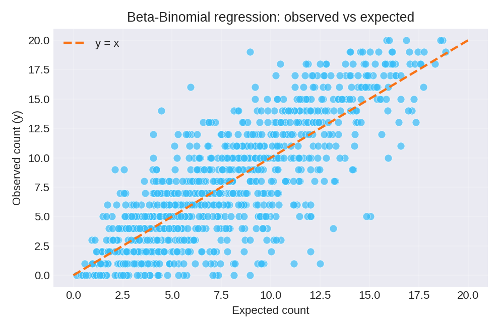
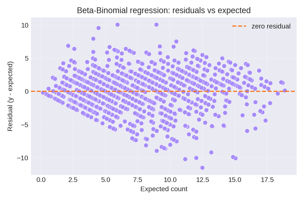
Results and Diagnostics

The posterior summaries recover the true parameters: $\beta_0 = 0.5$, $\beta_1 = 1.0$, and overdispersion $\rho = 0.2$. The diagnostic plots below compare observed counts with expected counts and show the residual pattern.

Observed counts versus expected counts with identity line — Observed counts $y_i$ versus expected counts $\hat{\mu}_i = N_i \hat{p}_i$.

Residuals versus expected counts — Residuals $y_i - \hat{\mu}_i$ versus expected counts.

To reproduce these figures locally, download the render_betabinomial_plots.py script and run it alongside the CSV dataset.