Beta Regression

Introduction

In this tutorial, we fit a Bayesian Beta regression model for data on the interval (0, 1). The Beta distribution is the natural choice when modeling proportions, rates, or probabilities where the response is continuous and bounded between 0 and 1.

The Beta likelihood uses a logit link function to ensure predictions stay within (0, 1), and includes a precision hyperparameter that controls the dispersion of the data around the mean.

The Model

We consider a Beta regression model with $n$ observations. For each observation $i = 1, \ldots, n$, the response $y_i \in (0, 1)$ is modeled as:

y_i \sim \text{Beta}(a_i, b_i)

where the shape parameters $a_i$ and $b_i$ are related to the mean $\mu_i$ and precision $\phi_i$ through:

a_i = \mu_i \phi_i, \qquad b_i = \phi_i (1 - \mu_i)

The mean and variance are:

\text{E}(y_i) = \mu_i, \qquad \text{Var}(y_i) = \frac{\mu_i(1-\mu_i)}{1+\phi_i}

Linear Predictor

The linear predictor $\eta_i$ links to the mean through a logit link function:

\eta_i = \beta_0 + \beta_1 z_i

The Beta distribution uses the logit link function (default):

\mu_i = \frac{\exp(\eta_i)}{1 + \exp(\eta_i)}

This ensures that the predicted mean is always in (0, 1).

Hyperparameters

The Beta likelihood has one hyperparameter: the precision parameter $\phi$. With a scale factor $s_i$:

\phi_i = s_i \exp(\theta)

where the prior is placed on $\theta$. The default prior is loggamma with parameters (1, 0.1).

Larger $\phi$ corresponds to smaller variance (more precision) for fixed $\mu$.

Dataset

The dataset contains $n = 1000$ observations with three columns:

Column	Description	Type
`y`	Response in (0, 1)	float
`z`	Covariate (predictor variable)	float
`w`	Scale factor for precision	float

dataset_beta_regression.csv

Download the CSV file and place it in your working directory.

Implementation in pyINLA

We fit the model using pyINLA with a varying precision through the scale parameter:

import pandas as pd
from pyinla import pyinla

# Load data
df = pd.read_csv('dataset_beta_regression.csv')
scale = df['w'].to_numpy()

# Define model: y ~ 1 + z (intercept + slope)
model = {
    'response': 'y',
    'fixed': ['1', 'z']
}

# Fit the Beta regression model
result = pyinla(
    model=model,
    family='beta',
    data=df,
    scale=scale
)

# View posterior summaries
print(result.summary_fixed)
print(result.summary_hyperpar)

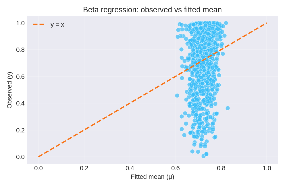
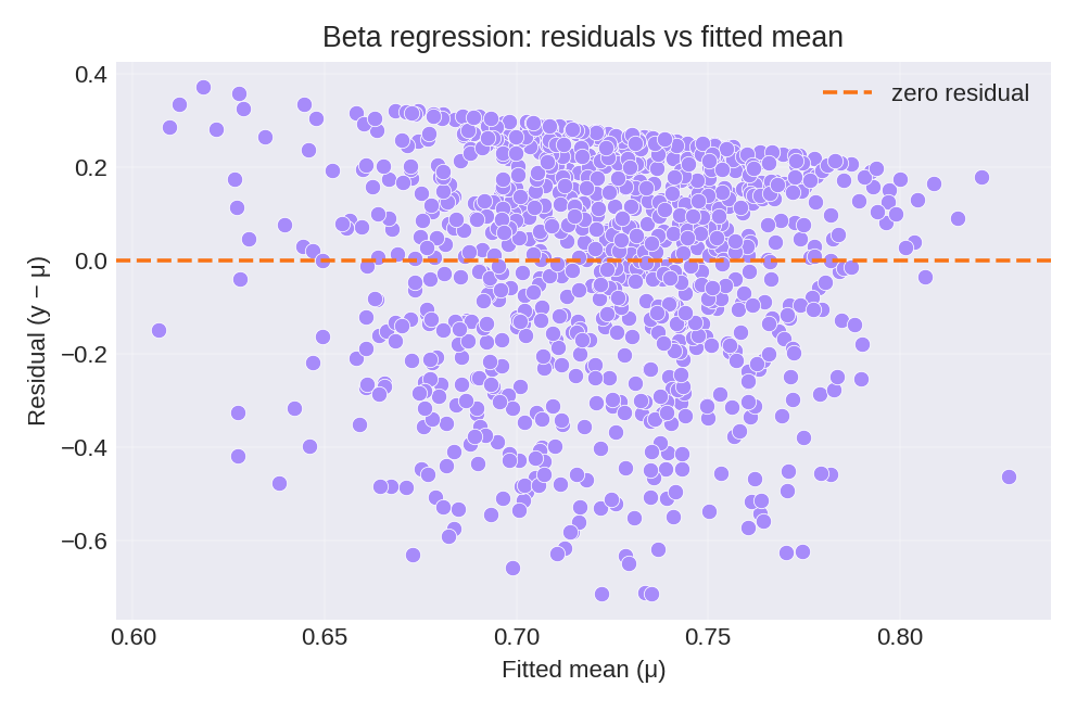
Results and Diagnostics

The posterior summaries provide estimates for $\beta_0$ and the precision hyperparameter $\theta$. The figures below show the model fit and residual diagnostics.

Observed values versus fitted mean with identity line — Observed values $y_i$ versus fitted mean $\hat{\mu}_i = \text{logit}^{-1}(\hat{\eta}_i)$.

Residuals versus fitted mean — Residuals $y_i - \hat{\mu}_i$ versus fitted mean.

To reproduce these figures locally, download the render_beta_plots.py script and run it alongside the CSV dataset.

Data Generation (Reference)

For reproducibility, the dataset was simulated from:

z_i \sim \mathcal{N}(0, 0.2), \quad w_i \sim \text{Uniform}(0.25, 0.75), \quad \phi_i = 5 w_i

with $\eta_i = 1 + z_i$, $\mu_i = \text{logit}^{-1}(\eta_i)$, $a_i = \mu_i \phi_i$, $b_i = \phi_i(1-\mu_i)$, and $y_i \sim \text{Beta}(a_i, b_i)$.

True parameter values: $\beta_0 = 1$, $\exp(\theta) = 5$.