Beta Regression with Censoring

Introduction

In some applications, observations very close to 0 or 1 are recorded as exactly 0 or 1 due to measurement limitations or rounding. The Beta distribution is defined on the open interval (0, 1), so exact 0s and 1s require special handling.

The Beta likelihood in pyINLA supports censoring: observations at or beyond a threshold are treated as censored rather than exact values.

Censoring Mechanism

A censoring threshold $\delta \in (0, 0.5)$ is specified:

Observations $y_i \leq \delta$ are treated as left-censored at 0
Observations $y_i \geq 1 - \delta$ are treated as right-censored at 1

For example, with $\delta = 0.05$:

y_i = \begin{cases} 0 & \text{if } y_i \leq 0.05 \\ 1 & \text{if } y_i \geq 0.95 \\ y_i & \text{otherwise} \end{cases}

Dataset

The dataset contains $n = 1000$ observations with two columns:

Column	Description	Type
`y`	Response (may include 0s and 1s)	float
`z`	Covariate (predictor variable)	float

dataset_beta_censored.csv

Download the CSV file and place it in your working directory.

Implementation in pyINLA

We fit the model using pyINLA with censoring enabled via beta.censor.value:

import pandas as pd
from pyinla import pyinla

# Load data
df = pd.read_csv('dataset_beta_censored.csv')
cens = 0.05  # censoring threshold

# Define model
model = {
    'response': 'y',
    'fixed': ['1', 'z']
}

# Control settings with censoring
control = {
    'family': {
        'beta.censor.value': cens
    }
}

# Fit the Beta regression model with censoring
result = pyinla(
    model=model,
    family='beta',
    data=df,
    control=control
)

# View posterior summaries
print(result.summary_fixed)
print(result.summary_hyperpar)

Extracting Results

The result object contains all posterior inference:

import numpy as np

# Fixed effects: posterior summaries for beta_0 and beta_1
print(result.summary_fixed)

# Extract posterior means
intercept = result.summary_fixed.loc['(Intercept)', 'mean']
slope = result.summary_fixed.loc['z', 'mean']

# Compute predicted probabilities (logit link)
eta_hat = intercept + slope * df['z'].to_numpy()
mu_hat = np.exp(eta_hat) / (1 + np.exp(eta_hat))

# Compute residuals
residuals = df['y'].to_numpy() - mu_hat

# Hyperparameters: precision phi
print(result.summary_hyperpar)

The summary_fixed DataFrame includes columns for mean, sd, 0.025quant, 0.5quant, 0.975quant, and mode.

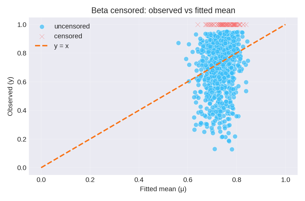
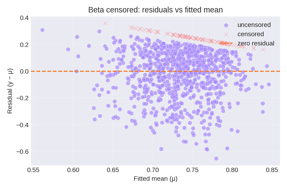
Results and Diagnostics

The posterior summaries provide estimates for $\beta_0$, $\beta_1$, and the precision $\phi$. Censored observations (at 0 and 1) are shown separately.

Observed vs fitted mean with censored points highlighted — Observed values $y_i$ versus fitted means $\hat{\mu}_i$. Censored points (at 0 or 1) shown in red.

Residuals versus fitted mean — Residuals $y_i - \hat{\mu}_i$ versus fitted means. Censored points shown in red.

To reproduce these figures locally, download the render_beta_plots.py script and run it alongside the CSV dataset.

Data Generation (Reference)

For reproducibility, the dataset was simulated with fixed precision $\phi = 5$:

z_i \sim \mathcal{N}(0, 0.2), \quad \eta_i = 1 + z_i, \quad \mu_i = \text{logit}^{-1}(\eta_i)

Then $y_i \sim \text{Beta}(\mu_i \phi, \phi(1-\mu_i))$ with censoring applied at $\delta = 0.05$.

True parameter values: $\beta_0 = 1$, $\phi = 5$.