Scottish Lip Cancer Disease Mapping
How do we identify areas with elevated disease risk after accounting for spatial correlation? Using a scaled BYM model with Poisson likelihood, we map relative risk across 56 Scottish districts, separate spatial and unstructured variation via two independent precision hyperparameters, and quantify the effect of an occupational covariate on lip cancer incidence.
Interpretable Insights from This Analysis
The scaled BYM disease mapping model decomposes regional disease risk into interpretable components, each with quantified uncertainty:
| Component | Parameter | Epidemiological Insight |
|---|---|---|
| Occupational exposure | $\beta_1$ (AFF effect) | Higher proportion of outdoor workers increases lip cancer risk |
| Spatial variation | $\sigma_{\text{spatial}}$ (spatial SD) | Controls the magnitude of spatially structured departures between neighboring districts |
| Unstructured variation | $\sigma_{\text{iid}}$ (IID SD) | Controls the magnitude of independent overdispersion in each district |
| Spatial fraction | $\phi$ (derived) | Over 90% of residual variation is spatially structured, not random noise |
| Relative risk map | $\theta_i = \exp(\eta_i)$ | Smoothed risk surface identifies high-risk areas in the Scottish Highlands |
Unlike crude standardised incidence ratios (SIR), the Bayesian spatial model borrows strength from neighboring districts, producing stable risk estimates even for areas with small populations.
Why Bayesian Disease Mapping?
Mapping disease rates across small areas is a core task in spatial epidemiology. Crude rates (observed/expected) are unreliable in sparsely populated areas due to high sampling variability. Bayesian spatial models address this by:
- Spatial smoothing: borrowing information from neighboring areas shrinks noisy estimates toward the local average, stabilising risk estimates in small populations.
- Structured + unstructured variation: the scaled BYM model separates spatially correlated variation (clustering) from independent noise (overdispersion) using two independent precision hyperparameters with PC priors.
- Covariate adjustment: fixed effects quantify how known risk factors (e.g. outdoor work) explain variation, with the random effects capturing residual spatial patterns.
- Exceedance probabilities: posterior distributions provide $P(\theta_i > 1 \mid \mathbf{y})$ for each area, enabling principled identification of disease hotspots.
INLA provides deterministic posterior approximations in seconds, making it practical for routine disease surveillance where MCMC would be too slow.
About the Data
The dataset records lip cancer cases observed in 56 Scottish districts during 1975-1980 (Clayton and Kaldor, 1987). It is one of the most widely used benchmarks in spatial epidemiology.
- 56 districts, 536 total observed cases
- Expected counts (E) based on age-sex standardisation against national rates
- Adjacency graph encoding which districts share a border
- 3 singleton islands (Orkney, Shetland, Western Isles) connected to their nearest mainland neighbor
| Variable | Description |
|---|---|
Y | Observed lip cancer cases in each district |
E | Expected cases (age-sex standardised) |
AFF | Proportion of population in agriculture, fishing, and forestry (outdoor work) |
idarea | District identifier (1-56) indexing the spatial random effect |
Download the data: scotland_data.csv, scotland.adj, scotland_districts.geojson
import pandas as pd
import numpy as np

data = pd.read_csv("scotland_data.csv")
data['idarea'] = np.arange(1, len(data) + 1)
data['SIR'] = data['Y'] / data['E']

print(f"Districts: {len(data)}")
print(f"Total observed cases: {data['Y'].sum()}")
print(f"Total expected cases: {data['E'].sum():.1f}")
print(f"AFF range: {data['AFF'].min():.2f} to {data['AFF'].max():.2f}")
Districts: 56
Total observed cases: 536
Total expected cases: 536.2
AFF range: 0.00 to 0.24The Statistical Model
For each district $i$, the observed count follows a Poisson distribution with an expected count offset:
where $\theta_i$ is the relative risk in district $i$, and $b_i$ is the scaled BYM random effect combining spatial and unstructured components:
Here $u_i$ is the ICAR (intrinsic conditional autoregressive) component encoding spatial dependence, $v_i \sim N(0, 1)$ is the IID component for overdispersion, and $s$ is the scaling factor (geometric mean of ICAR marginal variances) that standardises the spatial component. Unlike the BYM2 parameterization, the classic scaled BYM uses two separate precision hyperparameters for the spatial and IID components, and the spatial fraction $\phi$ is derived post hoc from posterior samples:
Model Components
| Parameter | Description | Prior |
|---|---|---|
| $\beta_0$ (Intercept) | Baseline log-relative-risk | $N(0, \sigma=31.62)$ (precision 0.001) |
| $\beta_1$ (AFF) | Effect of outdoor work proportion | $N(0, \sigma=31.62)$ (precision 0.001) |
| $\tau_{\text{iid}}$ | Precision of IID component | PC prior: $P(\sigma > 1) = 0.01$ |
| $\tau_{\text{spatial}}$ | Precision of ICAR component | PC prior: $P(\sigma > 1) = 0.01$ |
The PC (penalised complexity) priors (Simpson et al., 2017) shrink each standard deviation toward zero, encoding the principle that simpler models should be preferred unless the data support additional complexity. Setting $P(\sigma > 1) = 0.01$ means there is only a 1% prior probability that either standard deviation exceeds 1.
Step 1: Prepare the Adjacency Graph
The adjacency structure defines which districts are neighbors. Three island districts (Orkney, Shetland, Western Isles) have no neighbors in the original graph and must be connected to their nearest mainland district to form a single connected component:
import json
from scipy.sparse import diags, csc_matrix
from scipy.sparse.linalg import inv as sparse_inv

# Load district centroids from GeoJSON
with open("scotland_districts.geojson") as f:
    gj = json.load(f)

from shapely.geometry import shape
coords = np.array([shape(feat['geometry']).centroid.coords[0] for feat in gj['features']])

def compute_icar_scaling(adj):
    """Geometric mean of ICAR marginal variances (scaling factor)."""
    n = adj.shape[0]
    D = diags(adj.sum(axis=1))
    Q = D - csc_matrix(adj)
    # Add small constant for invertibility (sum-to-zero constraint)
    Q_inv = sparse_inv(csc_matrix(Q + np.ones((n, n)) / n)).toarray()
    marginal_var = np.diag(Q_inv)
    return np.exp(np.mean(np.log(marginal_var)))

def parse_adjacency(filepath):
    """Parse INLA-format adjacency file into a symmetric matrix."""
    with open(filepath, 'r') as f:
        lines = f.readlines()

    n = int(lines[0].strip())
    adj = np.zeros((n, n), dtype=float)

    for line in lines[1:]:
        parts = [int(x) for x in line.split()]
        node = parts[0] - 1  # 0-based
        for nb in parts[2:]:
            adj[node, nb - 1] = 1.0
            adj[nb - 1, node] = 1.0

    return adj

adj_matrix = parse_adjacency("scotland.adj")

# Connect islands to nearest mainland neighbor by centroid distance
# Orkney    -> Caithness
# Shetland  -> Caithness
# Western Isles -> Skye-Lochalsh

num_nb = adj_matrix.sum(axis=1)
singleton_idx = np.where(num_nb == 0)[0]
connected_idx = np.where(num_nb > 0)[0]

for s in singleton_idx:
    dists = np.sqrt(((coords[s] - coords[connected_idx])**2).sum(axis=1))
    nearest = connected_idx[np.argmin(dists)]
    adj_matrix[s, nearest] = 1
    adj_matrix[nearest, s] = 1
    print(f"Connected: {data['county'].iloc[s]} -> {data['county'].iloc[nearest]}")

# Save connected adjacency matrix in INLA format
import os
os.makedirs("output", exist_ok=True)
with open("output/scotland_connected.adj", "w") as f:
    n = adj_matrix.shape[0]
    f.write(f"{n}\n")
    for i in range(n):
        nbs = np.where(adj_matrix[i] > 0)[0] + 1  # 1-based
        f.write(f"{i+1} {len(nbs)} {' '.join(map(str, nbs))}\n")

scaling_factor = compute_icar_scaling(adj_matrix)
print(f"ICAR scaling factor: {scaling_factor:.6f}")
Connected: Orkney -> Caithness
Connected: Shetland -> Caithness
Connected: Western Isles -> Skye-Lochalsh
All 56 nodes now in one connected component
ICAR scaling factor: 0.625549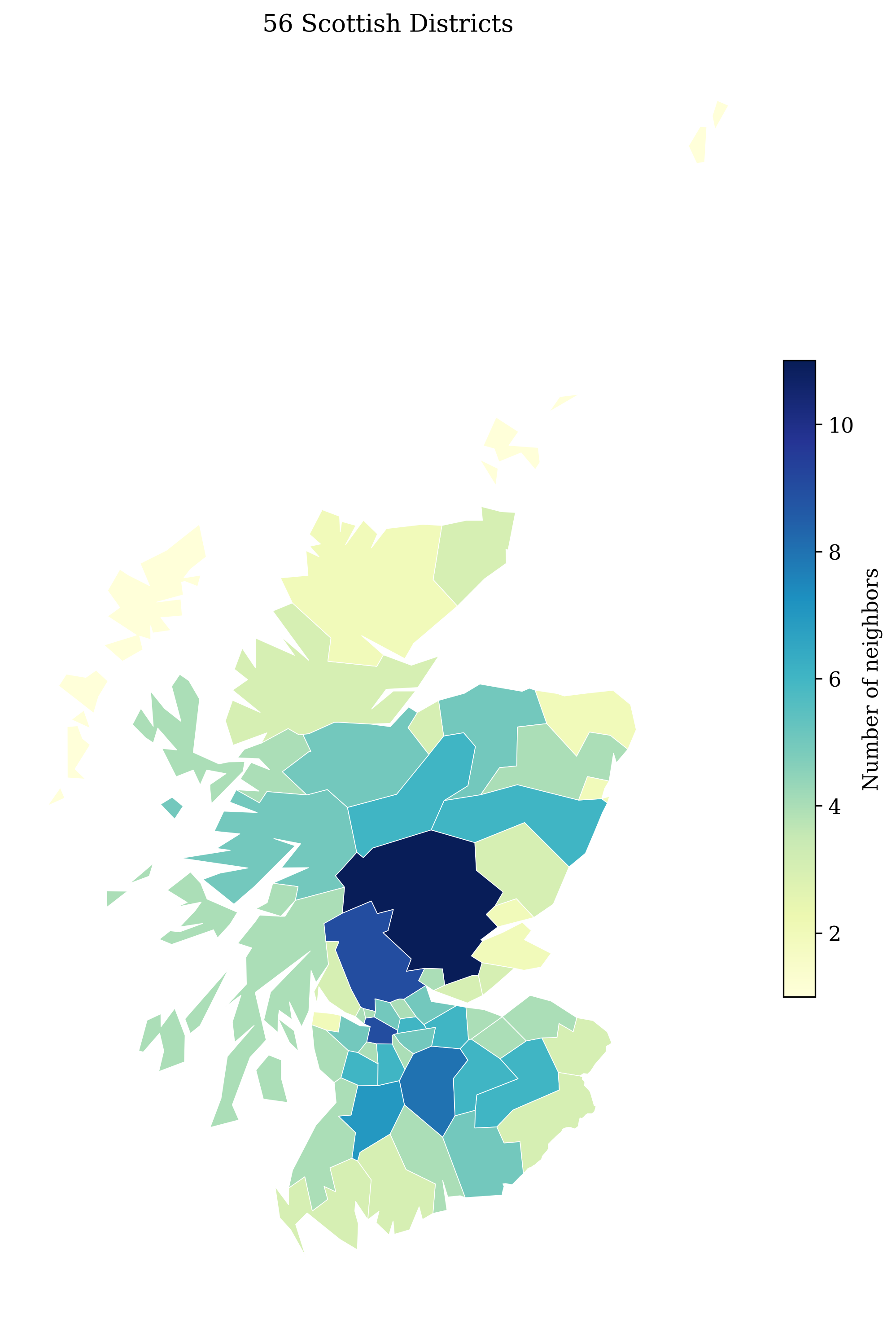
ICAR Scaling Factor
The scaling factor $s$ is computed as the geometric mean of the marginal variances of the ICAR precision matrix. Dividing the ICAR component by $\sqrt{s}$ standardises its variance, making the two precision hyperparameters comparable.
Step 2: Fit the Model with pyINLA
The model is specified as a Python dictionary. The response field names the outcome variable, fixed lists the intercept and covariates, and random defines the spatial random effect. Inside the random effect we set model='bym' with scale.model=True to use the scaled BYM, and assign PC priors to both hyperparameters: theta1 controls the IID precision and theta2 controls the spatial (ICAR) precision. The control block requests model comparison criteria (DIC, WAIC) and sets vague Gaussian priors (precision 0.001, i.e. $\sigma = 1/\sqrt{0.001} \approx 31.62$) on the fixed effects. The expected counts E are passed separately as an offset.
from pyinla import pyinla

model = {
    'response': 'Y',
    'fixed': ['1', 'AFF'],
    'random': [{
        'id': 'idarea',
        'model': 'bym',
        'graph': 'output/scotland_connected.adj',
        'scale.model': True,
        'hyper': {
            'theta1': {'prior': 'pc.prec', 'param': [1, 0.01]},
            'theta2': {'prior': 'pc.prec', 'param': [1, 0.01]}
        }
    }]
}

result = pyinla(
    model=model,
    family='poisson',
    data=data,
    E=data['E'].values,
    control={
        'compute': {'dic': True, 'waic': True, 'config': True, 'return_marginals': True},
        'fixed': {'prec.intercept': 0.001, 'prec': 0.001},
    }
)

print("Fixed effects:")
print(result.summary_fixed[['mean', 'sd', '0.025quant', '0.975quant']])
print("\nHyperparameters:")
print(result.summary_hyperpar[['mean', 'sd', '0.025quant', '0.975quant']])
Fixed effects:
mean sd 0.025quant 0.975quant
(Intercept) -0.264939 0.123755 -0.507560 -0.0208
AFF 4.217524 1.279915 1.662767 6.6975
Hyperparameters:
mean sd 0.025quant 0.975quant
Precision for idarea (iid component) 867.046703 6048.222795 8.009324 5845.17006
Precision for idarea (spatial component) 4.762687 1.855708 2.049507 9.23812PyINLA fits the full scaled BYM model in approximately 0.63 seconds, including computation of marginals, DIC, and WAIC.
Step 3: Interpret the Results
Occupational Exposure Effect
The AFF coefficient $\beta_1 \approx 4.22$ on the log scale indicates a strong positive association between outdoor work and lip cancer risk:
A 10 percentage-point increase in the proportion of outdoor workers is associated with approximately a 52% increase in relative risk. This is consistent with the known role of UV exposure in lip cancer aetiology.
Derived Spatial Fraction
Since the scaled BYM uses two separate precisions, the spatial fraction $\phi$ is derived from posterior hyperparameter samples rather than estimated directly:
from pyinla.sampling import inla_hyperpar_sample

hyp_samples = inla_hyperpar_sample(n=100000, result=result, intern=True).values
vv = np.exp(-hyp_samples)  # columns: 1/tau_iid, 1/tau_spatial
phi_samples = vv[:, 1] / vv.sum(axis=1)

print(f"Spatial fraction (phi): {phi_samples.mean():.3f}")
print(f"95% CI: [{np.percentile(phi_samples, 2.5):.3f}, {np.percentile(phi_samples, 97.5):.3f}]")
print(f"{phi_samples.mean()*100:.0f}% of residual variation is spatially structured")
Spatial fraction (phi): 0.919
95% CI: [0.646, 0.999]
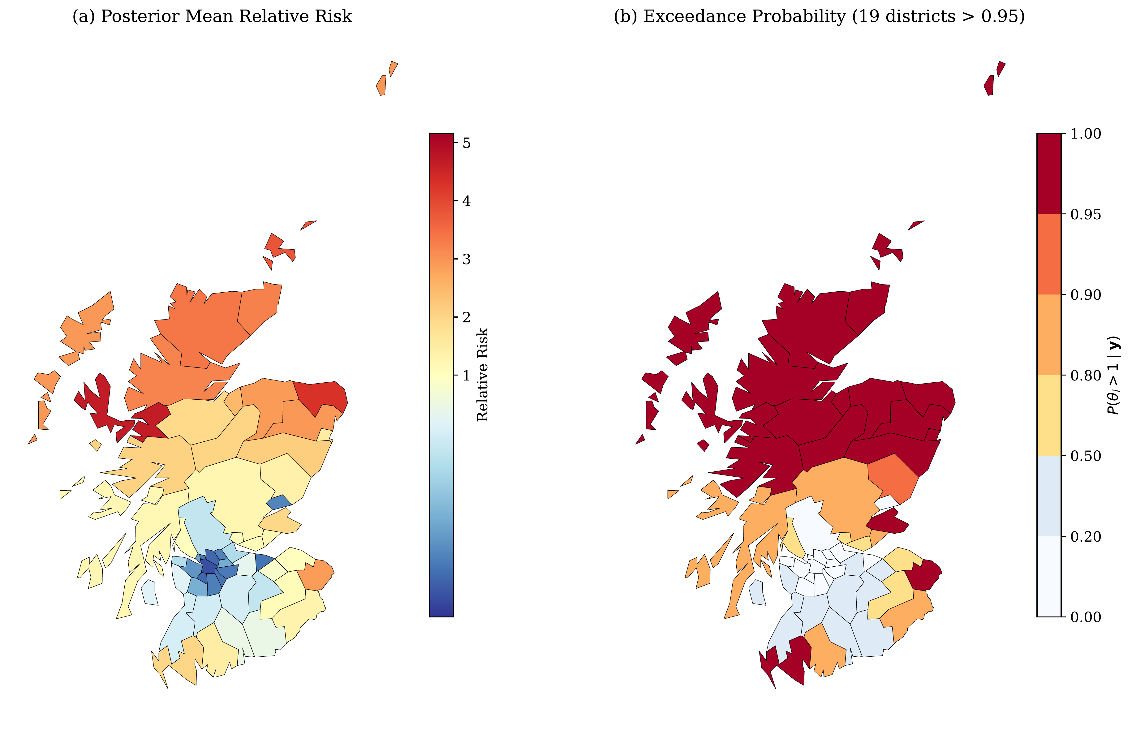
92% of residual variation is spatially structuredRelative Risk and Exceedance Probabilities
The fitted values from the Poisson model are on the log-relative-risk scale. We exponentiate to obtain $\theta_i$ and compute the exceedance probability $P(\theta_i > 1 \mid \mathbf{y})$ from the marginal posteriors:
from pyinla.marginal_utils import inla_pmarginal, inla_tmarginal

# Build results dataframe
results_df = data.copy()
fitted = result.summary_fitted_values
results_df['RR_mean'] = fitted['mean'].values
results_df['RR_lower'] = fitted['0.025quant'].values
results_df['RR_upper'] = fitted['0.975quant'].values

# Exceedance probability P(theta > 1 | y) from fitted marginals
marginals = result.marginals_fitted_values
results_df['exceed_prob'] = [
    1 - inla_pmarginal(np.array([1.0]), m)[0] for m in marginals
]

print(results_df[['county', 'SIR', 'RR_mean', 'exceed_prob']].head(10).to_string(index=False))
Relative Risk Map
The posterior mean relative risk $\theta_i$ and exceedance probability $P(\theta_i > 1 \mid \mathbf{y})$ are mapped across the 56 districts:
Top Risk Districts
top10 = results_df.nlargest(10, 'RR_mean')[['county', 'SIR', 'RR_mean', 'RR_lower', 'RR_upper']]
print(top10.to_string(index=False))
county SIR RR_mean RR_lower RR_upper
skye-lochalsh 6.429 4.660 2.617 7.797
banff-buchan 4.483 4.289 3.127 5.746
orkney 3.333 3.820 2.017 6.572
sutherland 2.778 3.342 1.701 5.895
caithness 3.667 3.227 1.873 5.218
ross-cromarty 3.488 3.195 1.997 4.870
shetland 3.043 2.957 1.453 5.391
western.isles 2.955 2.938 1.717 4.710
gordon 3.030 2.929 1.972 4.199
moray 3.210 2.895 2.011 4.052The model strongly smooths the extreme crude SIR for Skye-Lochalsh (6.4) down to 4.7, while pulling up risk estimates for island districts that borrow strength from their connected mainland neighbors.
MCMC Validation (PyMC/NUTS)
We fit the identical scaled BYM model using Hamiltonian Monte Carlo (NUTS) with 4 chains of 5,000 draws each. The PC prior $P(\sigma > 1) = 0.01$ translates to an Exponential($\lambda$) prior on the standard deviation with $\lambda = -\log(0.01) \approx 4.605$:
import pymc as pm
import pytensor.tensor as pt

pc_lambda = -np.log(0.01) / 1.0  # = 4.6052

with pm.Model(coords={'area': np.arange(56)}) as bym_model:
    beta0 = pm.Normal('beta0', mu=0, sigma=31.62)
    beta1 = pm.Normal('beta1', mu=0, sigma=31.62)

    sigma_spatial = pm.Exponential('sigma_spatial', lam=pc_lambda)
    sigma_iid = pm.Exponential('sigma_iid', lam=pc_lambda)

    v = pm.Normal('v', mu=0, sigma=1, dims='area')
    psi = pm.ICAR('psi', W=adj_matrix, dims='area')

    b = sigma_spatial / np.sqrt(scaling_factor) * psi + sigma_iid * v

    mu = pt.exp(logE + beta0 + beta1 * x + b)
    y_obs = pm.Poisson('y_obs', mu=mu, observed=y, dims='area')

    trace = pm.sample(5000, tune=3000, random_seed=42, cores=4,
                      target_accept=0.95)
Key validation results:
| Metric | PyINLA | MCMC | |Diff| |
|---|---|---|---|
| Intercept | $-0.2649$ | $-0.2610$ | $0.0039$ |
| AFF ($\beta_1$) | $4.2175$ | $4.1700$ | $0.0475$ |
| $\sigma_{\text{spatial}}$ | $0.4501$ | $0.4740$ | $0.0239$ |
| $\sigma_{\text{iid}}$ | $0.1202$ | $0.1192$ | $0.0010$ |
| $\phi$ (derived) | $0.919$ | $0.907$ | $0.012$ |
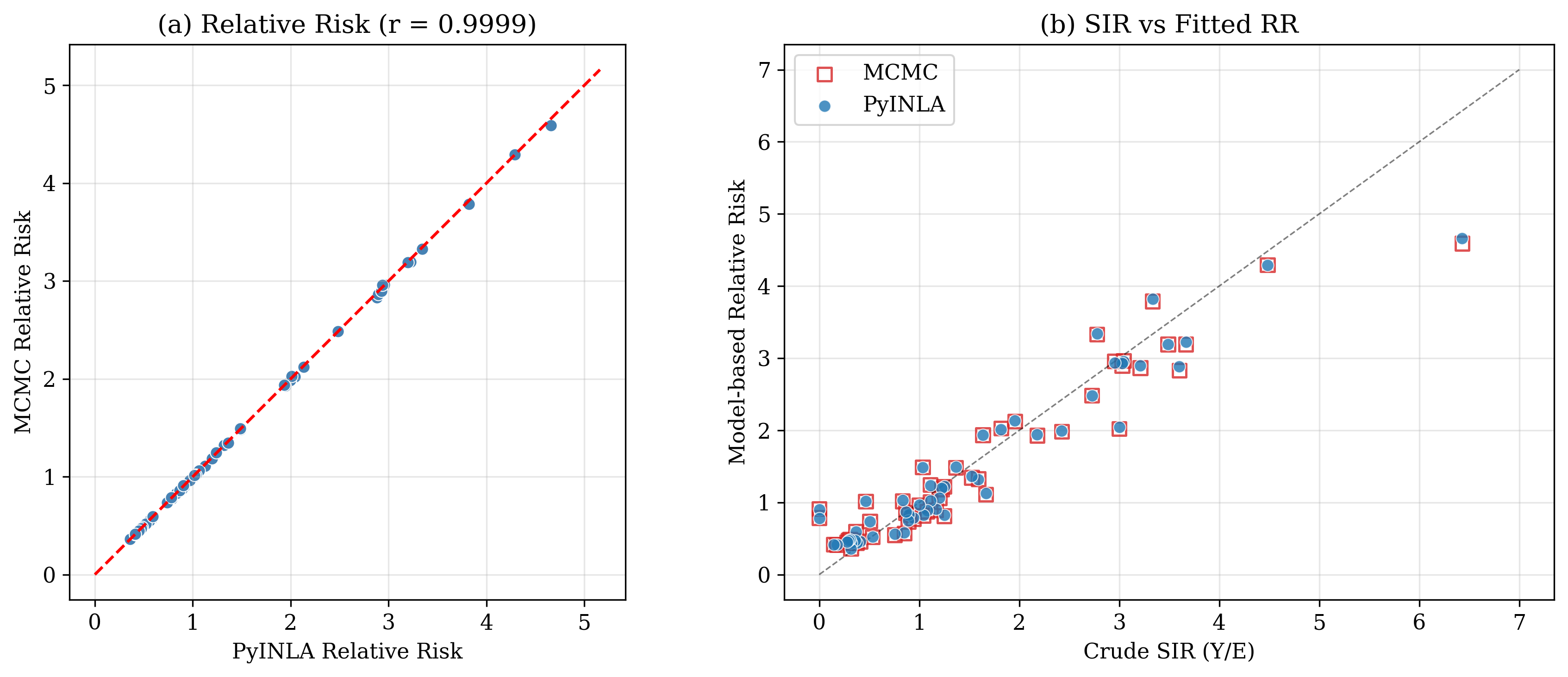
| RR correlation | Pearson $r = 0.9999$ | ||
- Relative risk correlation: Pearson $r = 0.9999$ across all 56 districts
- Fixed effects: AFF difference is only 0.04 posterior SD (excellent agreement)
- Speed: pyINLA runs in ~0.6 seconds vs ~120 seconds for MCMC (200x speedup)
Key Takeaways
- Scaled BYM disease mapping provides smoothed relative risk estimates that are far more reliable than crude SIRs, especially in sparsely populated areas.
- Outdoor work (AFF) is a strong predictor of lip cancer risk: a 10% increase in the proportion of outdoor workers corresponds to ~52% higher risk, consistent with UV exposure aetiology.
- 92% of residual variation is spatial: the derived spatial fraction $\phi$ confirms that neighboring districts share similar risk profiles beyond what AFF explains.
- PC priors on both precisions provide principled shrinkage toward simpler models. The very high IID precision (low $\sigma_{\text{iid}}$) indicates that nearly all residual variation is spatially structured.
- Exceedance probabilities identify disease hotspots with principled uncertainty quantification, providing actionable information for public health intervention.
- PyINLA matches MCMC to high precision ($r = 0.9999$) while running 200x faster, making it suitable for routine disease surveillance.
- Graph modification (connecting island singletons) is essential for the ICAR component and must be applied consistently across estimation methods.
Scaled BYM vs BYM2
The classic scaled BYM and the BYM2 (Riebler et al., 2016) are closely related but differ in parameterization:
| Feature | Scaled BYM | BYM2 |
|---|---|---|
| Hyperparameters | $\tau_{\text{iid}}, \tau_{\text{spatial}}$ (two precisions) | $\tau, \phi$ (one precision + mixing) |
| Spatial fraction | Derived post hoc from samples | Estimated directly as $\phi$ |
| Priors used here | PC prior on each precision | Gamma on $\tau$, Uniform on $\phi$ |
| Random effect | $\sigma_s / \sqrt{s} \cdot u_i + \sigma_v \cdot v_i$ | $\sigma(\sqrt{\phi/s} \cdot u_i + \sqrt{1-\phi} \cdot v_i)$ |
Both models produce similar relative risk estimates. The BYM2 parameterization makes $\phi$ directly interpretable and enables prior specification on the spatial fraction. The scaled BYM with PC priors provides stronger regularization through principled shrinkage of each variance component independently.
References
- Clayton, D. and Kaldor, J. (1987). "Empirical Bayes estimates of age-standardized relative risks for use in disease mapping." Biometrics, 43(3), 671-681.
- Riebler, A., Sorbye, S.H., Simpson, D. and Rue, H. (2016). "An intuitive Bayesian spatial model for disease mapping that accounts for scaling." Statistical Methods in Medical Research, 25(4), 1145-1165.
- Simpson, D., Rue, H., Riebler, A., Martins, T.G. and Sorbye, S.H. (2017). "Penalising model component complexity: A principled, practical approach to constructing priors." Statistical Science, 32(1), 1-28.
- Konstantinoudis, G., Cameletti, M., Gomez-Rubio, V., Gomez, I.L., Pirani, M., Baio, G., Larrauri, A., Riou, J., Egger, M., Vineis, P. and Blangiardo, M. (2021). "Regional excess mortality during the 2020 COVID-19 pandemic in five European countries." Nature Communications, 13(1), 482.
- Rue, H., Martino, S. and Chopin, N. (2009). "Approximate Bayesian inference for latent Gaussian models using integrated nested Laplace approximations." Journal of the Royal Statistical Society: Series B, 71(2), 319-392.