Modeling Airline Passenger Seasonality
How do we decompose a time series into trend and seasonal components? Using Bayesian seasonal models with INLA, we analyze the classic AirPassengers dataset to extract the underlying structure of monthly international airline traffic from 1949 to 1960.
Interpretable Insights from This Analysis
The Seasonal model decomposes the time series into two interpretable components, each with quantified uncertainty:
| Component | Parameter | Business Insight |
|---|---|---|
| Long-term trend | $\alpha_{\text{year}}$ (year effects) | Market grew 3.8x from 128k to 480k passengers (1949-1960) |
| Seasonal peak | $u_m$ (seasonal effects) | July and August run ~22% above yearly average |
| Seasonal trough | $u_m$ (seasonal effects) | November runs ~18% below yearly average |
| Capacity planning | $\exp(u_{\text{Jul}} - u_{\text{Nov}})$ | Summer demand estimated roughly 40-50% higher than late autumn (model-based) |
Unlike black-box forecasting methods, Bayesian models provide direct parameter estimates with credible intervals, enabling not just prediction, but explanation and decision-making under uncertainty.
Why Study Seasonal Patterns?
Many real-world time series exhibit seasonal patterns: regular fluctuations that repeat over a fixed period. Understanding these patterns is crucial for:
- Forecasting: predicting future values requires capturing the seasonal structure
- Trend extraction: separating the long-term trend from seasonal noise
- Anomaly detection: identifying unusual observations after accounting for expected seasonal variation
- Resource planning: businesses need to anticipate seasonal demand fluctuations
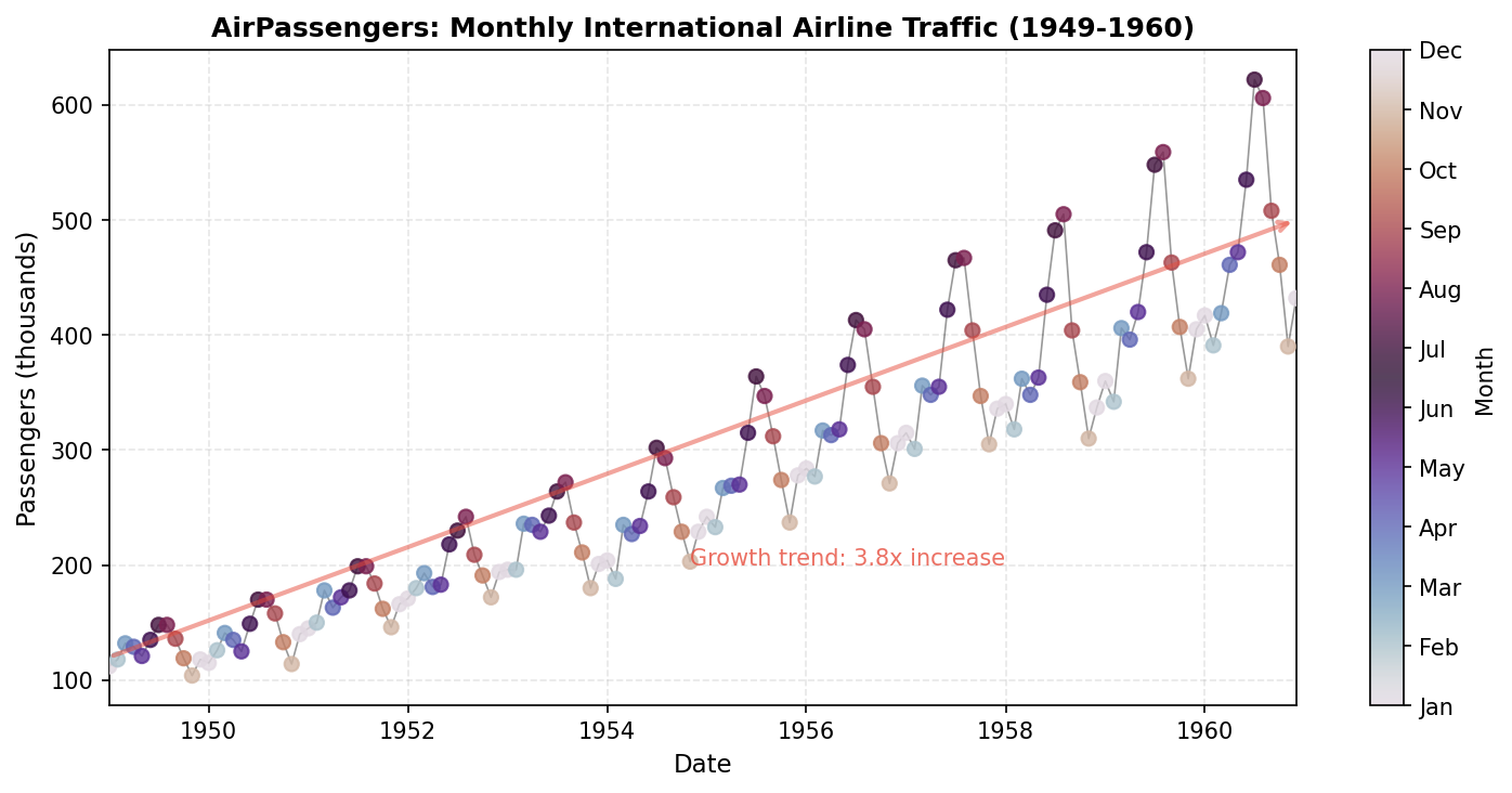
The AirPassengers dataset is one of the most famous time series datasets in statistics, first analyzed by Box, Jenkins, and Reinsel (1976). It demonstrates clear multiplicative seasonality with an upward trend, perfect for illustrating seasonal decomposition techniques.
About the Data
The AirPassengers dataset records the total monthly international airline passengers (in thousands) from January 1949 to December 1960. Key characteristics include:
- 144 observations: 12 years of monthly data
- Strong upward trend: air travel grew rapidly during this period
- Clear seasonality: peak travel in summer months (June-August)
- Multiplicative pattern: seasonal amplitude increases with the level
For modeling, we transform the data to a data frame with explicit time indices:
| Variable | Description |
|---|---|
passengers | Number of passengers (thousands) |
year | Year (1949-1960) as factor for trend |
month | Month of year (1-12) |
time | Time index (1-144) |
The Seasonal Model
We model the log-transformed passengers as an additive decomposition into a year-level baseline and a repeating month-of-year seasonal effect (Gomez-Rubio, 2020):
where the linear predictor $\eta_t$ includes a year effect (trend) and a seasonal component indexed by month-of-year:
Here $\alpha_{\text{year}(t)}$ is a fixed effect for the calendar year, and $u_{\text{month}(t)}$ is a seasonal random effect with $\text{month}(t) \in \{1, \ldots, 12\}$. The first 10 observations illustrate how the indices map:
| $t$ | Date | $y_t$ | Year effect | Seasonal index |
|---|---|---|---|---|
| 1 | Jan 1949 | 112 | $\alpha_{1949}$ | $u_1$ |
| 2 | Feb 1949 | 118 | $\alpha_{1949}$ | $u_2$ |
| 3 | Mar 1949 | 132 | $\alpha_{1949}$ | $u_3$ |
| 4 | Apr 1949 | 129 | $\alpha_{1949}$ | $u_4$ |
| 5 | May 1949 | 121 | $\alpha_{1949}$ | $u_5$ |
| 6 | Jun 1949 | 135 | $\alpha_{1949}$ | $u_6$ |
| 7 | Jul 1949 | 148 | $\alpha_{1949}$ | $u_7$ |
| 8 | Aug 1949 | 148 | $\alpha_{1949}$ | $u_8$ |
| 9 | Sep 1949 | 136 | $\alpha_{1949}$ | $u_9$ |
| 10 | Oct 1949 | 119 | $\alpha_{1949}$ | $u_{10}$ |
Note: $\alpha$ changes with each calendar year (1949, 1950, ...), while $u_m$ cycles through months $m \in \{1, \ldots, 12\}$ repeatedly.
Let $\mathbf{u} = (u_1, \ldots, u_{12})^\top$ denote the month-of-year seasonal effects. In INLA's seasonal specification, $u_m$ represents a repeating annual deviation (on the log scale) associated with month $m$. Because the overall level is captured by the year fixed effects, the seasonal effects are interpreted relative to that baseline and are typically close to centered, though not necessarily constrained to sum exactly to zero.
Note: The seasonal model has constr=FALSE by default in R-INLA/pyINLA. To impose a strict sum-to-zero constraint, set 'constr': True in the model specification.
Hyperparameters
| Parameter | Description | Default Prior |
|---|---|---|
| Observation precision ($\tau_\varepsilon$) | Precision of Gaussian likelihood | log-Gamma(1, 0.00005) |
| Seasonal precision ($\tau$) | Precision of seasonal effect | log-Gamma(1, 0.00005) |
Step 1: Data Preparation
We create the dataset from scratch to match the AirPassengers data:
import numpy as np
import pandas as pd

# AirPassengers data (monthly totals in thousands)
passengers = [
    112, 118, 132, 129, 121, 135, 148, 148, 136, 119, 104, 118,  # 1949
    115, 126, 141, 135, 125, 149, 170, 170, 158, 133, 114, 140,  # 1950
    145, 150, 178, 163, 172, 178, 199, 199, 184, 162, 146, 166,  # 1951
    171, 180, 193, 181, 183, 218, 230, 242, 209, 191, 172, 194,  # 1952
    196, 196, 236, 235, 229, 243, 264, 272, 237, 211, 180, 201,  # 1953
    204, 188, 235, 227, 234, 264, 302, 293, 259, 229, 203, 229,  # 1954
    242, 233, 267, 269, 270, 315, 364, 347, 312, 274, 237, 278,  # 1955
    284, 277, 317, 313, 318, 374, 413, 405, 355, 306, 271, 306,  # 1956
    315, 301, 356, 348, 355, 422, 465, 467, 404, 347, 305, 336,  # 1957
    340, 318, 362, 348, 363, 435, 491, 505, 404, 359, 310, 337,  # 1958
    360, 342, 406, 396, 420, 472, 548, 559, 463, 407, 362, 405,  # 1959
    417, 391, 419, 461, 472, 535, 622, 606, 508, 461, 390, 432   # 1960
]

# Create year labels (1949-1960) as string factors
years = []
for year in range(1949, 1961):
    years.extend([str(year)] * 12)

# Create month indices (1-12, repeated for each year)
months = list(range(1, 13)) * 12

# Create the dataframe
df = pd.DataFrame({
    'passengers': passengers,
    'year': years,
    'month': months,
    'time': range(1, 145)
})

# Log-transform the response for additive seasonality
df['log_passengers'] = np.log(df['passengers'])

print(df.head(15))
print(f"\nTotal observations: {len(df)}")
print(f"Years: 1949-1960")
print(f"Monthly range: {min(passengers)} to {max(passengers)} thousand")
passengers year month time log_passengers
0 112 1949 1 1 4.718499
1 118 1949 2 2 4.770685
2 132 1949 3 3 4.882802
3 129 1949 4 4 4.859812
4 121 1949 5 5 4.795791
5 135 1949 6 6 4.905275
6 148 1949 7 7 4.997212
7 148 1949 8 8 4.997212
8 136 1949 9 9 4.912655
9 119 1949 10 10 4.779123
10 104 1949 11 11 4.644391
11 118 1949 12 12 4.770685
12 115 1950 1 13 4.744932
13 126 1950 2 14 4.836282
14 141 1950 3 15 4.948760
Total observations: 144
Years: 1949-1960
Monthly range: 104 to 622 thousandVisualize the Data
import matplotlib.pyplot as plt

# Create date index for plotting
dates = pd.date_range('1949-01', periods=144, freq='M')
month_names = ['Jan', 'Feb', 'Mar', 'Apr', 'May', 'Jun',
               'Jul', 'Aug', 'Sep', 'Oct', 'Nov', 'Dec']

fig, ax = plt.subplots(figsize=(10, 5))
scatter = ax.scatter(dates, df['passengers'], c=df['month'],
                     cmap='twilight', s=40, alpha=0.8, zorder=3)
ax.plot(dates, df['passengers'], 'k-', lw=0.8, alpha=0.4, zorder=2)

cbar = plt.colorbar(scatter, ax=ax, ticks=range(1, 13))
cbar.set_label('Month')
cbar.set_ticklabels(month_names)

ax.set_xlabel('Date')
ax.set_ylabel('Passengers (thousands)')
ax.set_title('AirPassengers: Monthly International Airline Traffic (1949-1960)')
ax.grid(True, alpha=0.3, linestyle='--')

ax.annotate('', xy=(dates[-1], 500), xytext=(dates[0], 120),
            arrowprops=dict(arrowstyle='->', color='#e74c3c', lw=2, alpha=0.5))
ax.text(dates[70], 200, 'Growth trend: 3.8x increase', color='#e74c3c', alpha=0.8)

plt.tight_layout()
plt.savefig('data_overview.png', dpi=150, bbox_inches='tight')
Step 2: Fit the Seasonal Model
We fit a model with year as a fixed effect (to capture the trend) and a seasonal random effect with period 12:
from pyinla import pyinla

# Define the model structure
model = {
    'response': 'log_passengers',
    'fixed': ['-1', 'year'],  # No global intercept, year-specific means
    'random': [
        {'id': 'month', 'model': 'seasonal', 'season.length': 12}
    ]
}

# Fit the model
result = pyinla(
    model=model,
    family='gaussian',
    data=df
)

# View the results
print("Fixed Effects (Year Means on Log Scale):")
print(result.summary_fixed)

print("\nHyperparameters:")
print(result.summary_hyperpar)
mean sd 0.025quant 0.5quant 0.975quant mode kld
year1949 4.854912 0.033542 4.786759 4.854940 4.922767 4.854903 0.034547
year1950 4.949558 0.033542 4.881405 4.949585 5.017413 4.949549 0.034547
year1951 5.150143 0.033542 5.081990 5.150171 5.217998 5.150134 0.034547
year1952 5.295964 0.033542 5.227811 5.295992 5.363819 5.295955 0.034547
year1953 5.427430 0.033542 5.359277 5.427458 5.495285 5.427421 0.034547
year1954 5.485270 0.033542 5.417118 5.485298 5.553126 5.485261 0.034547
year1955 5.658002 0.033542 5.589849 5.658030 5.725857 5.657993 0.034547
year1956 5.803162 0.033542 5.735009 5.803190 5.871017 5.803153 0.034547
year1957 5.917106 0.033542 5.848953 5.917133 5.984961 5.917097 0.034547
year1958 5.949315 0.033542 5.881163 5.949343 6.017171 5.949306 0.034547
year1959 6.067101 0.033542 5.998948 6.067129 6.134956 6.067092 0.034547
year1960 6.172948 0.033542 6.104796 6.172976 6.240804 6.172939 0.034547 mean sd 0.025quant 0.5quant 0.975quant mode
Precision for the Gaussian observations 697.827719 89.109212 536.793574 692.918503 887.010843 684.568696
Precision for month 4.938363 5.392276 0.333190 3.250105 19.256532 0.910461Step 3: Interpret the Results
Year Effects (Trend)
The year coefficients $\alpha_{\text{year}}$ are estimated on the log scale. To convert back to the original passenger scale, we exponentiate:
For example, for 1949 we have $\alpha_{1949} = 4.855$, so:
Note: Why geometric mean? (click to expand)
Arithmetic mean: $\bar{y} = \frac{1}{n}\sum_{i=1}^{n} y_i$ (sum and divide)
Geometric mean: $\tilde{y} = \exp\left(\frac{1}{n}\sum_{i=1}^{n} \log y_i\right)$ (average logs, exponentiate)
Since $\exp(\alpha) = \exp(\mathbb{E}[\log y])$, we get the geometric mean $\tilde{y}$, not arithmetic $\bar{y}$. Jensen's inequality: $\tilde{y} \leq \bar{y}$.
# Convert log-scale year means to original scale
year_means = result.summary_fixed['mean']
print("Average monthly passengers by year (thousands):")
for year_label, log_mean in year_means.items():
    print(f"  {year_label.replace('year', '')}: {np.exp(log_mean):.0f}")
Average monthly passengers by year (thousands):
1949: 128
1950: 141
1951: 172
1952: 200
1953: 228
1954: 241
1955: 287
1956: 331
1957: 371
1958: 383
1959: 431
1960: 480Passengers nearly quadrupled from 1949 to 1960 (3.8x growth), reflecting the rapid growth of commercial aviation.
Seasonal Effects
The seasonal random effects capture the monthly pattern within each year:
# Extract seasonal effects (first 12 values = monthly pattern)
seasonal = result.summary_random['month']
first_year = seasonal.iloc[:12][['mean', '0.025quant', '0.975quant']].copy()
first_year.columns = ['Effect', 'Lower', 'Upper']

month_names = ['Jan', 'Feb', 'Mar', 'Apr', 'May', 'Jun',
               'Jul', 'Aug', 'Sep', 'Oct', 'Nov', 'Dec']
first_year['Month'] = month_names

print("Seasonal Effects (deviations from year mean):")
print(first_year[['Month', 'Effect', 'Lower', 'Upper']].to_string(index=False))
Seasonal Effects (deviations from year mean):
Month Effect Lower Upper
Jan -0.159375 -0.227468 -0.091198
Feb -0.171319 -0.239346 -0.103270
Mar -0.031091 -0.098980 0.036921
Apr -0.052377 -0.120124 0.015620
May -0.044802 -0.112390 0.023216
Jun 0.087265 0.019847 0.155333
Jul 0.201182 0.133886 0.269269
Aug 0.201991 0.134712 0.270008
Sep 0.067588 0.000224 0.135450
Oct -0.060295 -0.127786 0.007387
Nov -0.193776 -0.261374 -0.126237
Dec -0.069798 -0.137420 -0.002301Trend and Seasonality Together
Now we can visualize both components side by side:
# Plot year effects (trend) and seasonal pattern side by side
year_effects = result.summary_fixed
years_list = [int(y.replace('year', '')) for y in year_effects.index]  # strips 'year' prefix from e.g. 'year1949'
year_means = np.exp(year_effects['mean'].values)
year_lower = np.exp(year_effects['0.025quant'].values)
year_upper = np.exp(year_effects['0.975quant'].values)

fig, axes = plt.subplots(1, 2, figsize=(12, 4.5))

# Left: Year effects on original scale with 95% CI
axes[0].fill_between(years_list, year_lower, year_upper, alpha=0.3, color='#3498db')
axes[0].plot(years_list, year_means, 'o-', color='#2c3e50', lw=2, markersize=8)
axes[0].set_xlabel('Year')
axes[0].set_ylabel('Average Passengers (thousands)')
axes[0].set_title('Estimated Yearly Mean (with 95% CI)')
axes[0].grid(True, alpha=0.3, linestyle='--')
axes[0].set_xticks(years_list)
axes[0].set_xticklabels(years_list, rotation=45)
axes[0].annotate(f'{year_means[0]:.0f}k', xy=(years_list[0], year_means[0]),
                 xytext=(years_list[0]+0.5, year_means[0]+30), fontsize=9)
axes[0].annotate(f'{year_means[-1]:.0f}k', xy=(years_list[-1], year_means[-1]),
                 xytext=(years_list[-1]-1.5, year_means[-1]+30), fontsize=9, ha='right')

# Right: Seasonal pattern (% deviation from year mean)
seasonal_vals = first_year['Effect'].values
multipliers = np.exp(seasonal_vals)
pct_dev = (multipliers - 1) * 100
colors = ['#3498db' if m > 1 else '#e74c3c' for m in multipliers]
bars = axes[1].bar(month_names, pct_dev, color=colors, edgecolor='white', linewidth=1)
axes[1].axhline(0, color='k', lw=0.8)
axes[1].set_xlabel('Month')
axes[1].set_ylabel('% Deviation from Year Mean')
axes[1].set_title('Seasonal Pattern (% above/below yearly average)')
axes[1].grid(True, alpha=0.3, linestyle='--', axis='y')
axes[1].tick_params(axis='x', rotation=45)

for bar, m in zip(bars, multipliers):
    if abs(m - 1) > 0.15:
        height = (m - 1) * 100
        axes[1].annotate(f'{height:+.0f}%',
                         xy=(bar.get_x() + bar.get_width() / 2, height),
                         xytext=(0, 3 if height >= 0 else -12),
                         textcoords="offset points", ha='center',
                         va='bottom' if height >= 0 else 'top', fontsize=9, fontweight='bold')

plt.tight_layout()
plt.savefig('trend_and_seasonality.png', dpi=150, bbox_inches='tight')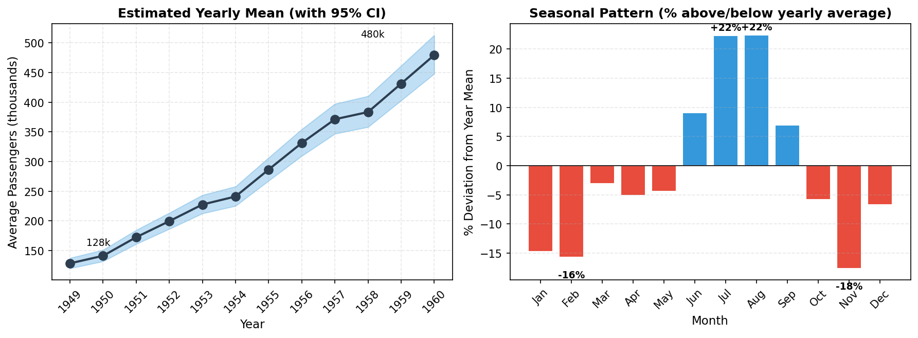
# Bar chart of seasonal effects with value labels
seasonal_vals = first_year['Effect'].values
colors = ['#3498db' if e > 0 else '#e74c3c' for e in seasonal_vals]

fig, ax = plt.subplots(figsize=(10, 5))
bars = ax.bar(month_names, seasonal_vals, color=colors, edgecolor='white', linewidth=1.5)

for bar, val in zip(bars, seasonal_vals):
    height = bar.get_height()
    ax.annotate(f'{val:+.2f}',
                xy=(bar.get_x() + bar.get_width() / 2, height),
                xytext=(0, 3 if height >= 0 else -12),
                textcoords="offset points", ha='center',
                va='bottom' if height >= 0 else 'top', fontsize=9, fontweight='bold')

ax.axhline(0, color='k', lw=0.8)
ax.set_ylabel('Effect (log scale)')
ax.set_xlabel('Month')
ax.set_title('Seasonal Effects (deviations from year mean)')
ax.grid(True, alpha=0.3, linestyle='--', axis='y')
ax.set_ylim(-0.3, 0.35)

plt.tight_layout()
plt.savefig('seasonal_effects.png', dpi=150, bbox_inches='tight')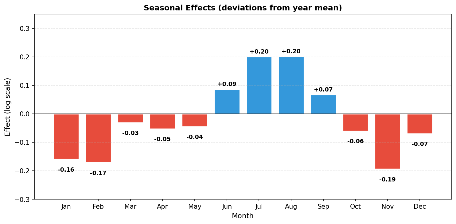
Interpretation:
- July-August peak: Highest travel (~22% above yearly average)
- November trough: Lowest travel (~18% below yearly average)
- Summer dominance: June-September all show positive effects
- Winter lull: January-February and November show the largest negative effects
Multiplicative Interpretation
Since the model is on the log scale, a month effect $u_m$ corresponds to a multiplicative factor $\exp(u_m)$ on the original scale:
The term $\exp(u_m)$ is a multiplier relative to the yearly baseline. To express as a percentage change:
Why subtract 1? When there is no seasonal effect ($u_m = 0$), the multiplier is $\exp(0) = 1$, meaning "100% of baseline" or "no change." Subtracting 1 converts the multiplier to a deviation: $1.22 - 1 = 0.22 = +22\%$ above baseline.
For example, if $u_{\text{Jul}} \approx 0.20$, then July is associated with an expected multiplier of $\exp(0.20) \approx 1.22$, i.e., about a 22% increase relative to the year baseline.
Comparing Two Months
Using the Seasonal model results, a direct comparison between two months $m_1$ and $m_2$ on the original scale is given by:
# Compare July (index 6) vs November (index 10) using seasonal model
u_jul = first_year.loc[6, 'Effect']  # 0.201
u_nov = first_year.loc[10, 'Effect']  # -0.194

ratio = np.exp(u_jul - u_nov)
print(f"July effect: {u_jul:+.3f}")
print(f"November effect: {u_nov:+.3f}")
print(f"Difference: {u_jul - u_nov:.3f}")
print(f"Ratio exp({u_jul - u_nov:.3f}) = {ratio:.2f}")
print(f"July demand is roughly {(ratio - 1) * 100:.0f}% higher than November")
July effect: +0.201
November effect: -0.194
Difference: 0.395
Ratio exp(0.395) = 1.48
July demand is roughly 48% higher than NovemberNote: This is a model-based point estimate from the Seasonal model. For rigorous inference, report the posterior credible interval for $\exp(u_{\text{Jul}} - u_{\text{Nov}})$.
# Convert seasonal effects to multiplicative factors
print("Monthly multipliers (relative to year average):")
for month, effect in zip(month_names, first_year['Effect']):
    multiplier = np.exp(effect)
    print(f"  {month}: {multiplier:.3f} ({(multiplier-1)*100:+.1f}%)")
Monthly multipliers (relative to year average):
Jan: 0.853 (-14.7%)
Feb: 0.843 (-15.7%)
Mar: 0.969 (-3.1%)
Apr: 0.949 (-5.1%)
May: 0.956 (-4.4%)
Jun: 1.091 (+9.1%)
Jul: 1.223 (+22.3%)
Aug: 1.224 (+22.4%)
Sep: 1.070 (+7.0%)
Oct: 0.941 (-5.9%)
Nov: 0.824 (-17.6%)
Dec: 0.933 (-6.7%)Step 4: Model Fit Assessment
How well does the seasonal model fit the observed data? We compare fitted values $\hat{y}_t = \exp(\hat{\eta}_t)$ to observed passengers using descriptive metrics:
Coefficient of determination (R²) measures the proportion of variance explained by the model:
$R^2 = 1$ means perfect fit; $R^2 = 0$ means the model does no better than predicting the mean. Note: This is an in-sample measure and should not be interpreted as out-of-sample forecast accuracy.
Root mean squared error (RMSE) measures average prediction error in original units:
# Get fitted values on original scale (use .values to avoid index mismatch)
fitted_log = result.summary_fitted_values['mean'].values
fitted = np.exp(fitted_log)  # Back-transform from log scale
observed = df['passengers'].values

# Compute fit statistics
residuals = observed - fitted
ss_res = np.sum(residuals**2)
ss_tot = np.sum((observed - observed.mean())**2)
r_squared = 1 - ss_res / ss_tot
rmse = np.sqrt(np.mean(residuals**2))

print(f"R² = {r_squared:.4f}")
print(f"RMSE = {rmse:.1f} thousand passengers")
R² = 0.9925
RMSE = 10.4 thousand passengersVisualizing the Fit
import matplotlib.pyplot as plt

# Create time index for x-axis
dates = pd.date_range('1949-01', periods=144, freq='M')

fig, axes = plt.subplots(2, 1, figsize=(10, 6), gridspec_kw={'height_ratios': [2, 1]})

# Top: Observed vs Fitted
axes[0].scatter(dates, observed, s=25, alpha=0.6, c='#2c3e50', label='Observed', zorder=3)
axes[0].plot(dates, fitted, color='#e74c3c', lw=2, label='Fitted', zorder=4)
axes[0].fill_between(dates, fitted, alpha=0.1, color='#e74c3c')
axes[0].set_ylabel('Passengers (thousands)')
axes[0].legend(loc='upper left', framealpha=0.95)
axes[0].set_title('Seasonal Model: Observed vs Fitted')
axes[0].grid(True, alpha=0.3, linestyle='--')

# Bottom: Residuals
colors = ['#27ae60' if r >= 0 else '#e74c3c' for r in residuals]
axes[1].bar(dates, residuals, width=25, color=colors, alpha=0.7, edgecolor='none')
axes[1].axhline(0, color='k', lw=0.8)
axes[1].set_ylabel('Residual')
axes[1].set_xlabel('Date')
axes[1].set_title('Residuals over Time')
axes[1].grid(True, alpha=0.3, linestyle='--')

plt.tight_layout()
plt.savefig('model_fit.png', dpi=150)
The seasonal model achieves R² ≈ 0.99 for this dataset, and fitted values closely track observations (residuals on the order of ±10 thousand passengers). These summaries describe in-sample agreement only; predictive performance should be assessed with out-of-sample validation or posterior predictive checks.
Alternative: AR(1) Model for Autocorrelation
We can also model the temporal dependence using an AR(1) random effect instead of the seasonal model:
# Model with AR1 instead of seasonal
model_ar1 = {
    'response': 'log_passengers',
    'fixed': ['-1', 'year'],
    'random': [
        {'id': 'time', 'model': 'ar1'}
    ]
}

result_ar1 = pyinla(
    model=model_ar1,
    family='gaussian',
    data=df
)

print("AR1 Model Hyperparameters:")
print(result_ar1.summary_hyperpar)
mean sd 0.025quant 0.5quant 0.975quant mode
Precision for the Gaussian observations 24897.6892 24949.6049 2243.0771 17397.69 91151.6002 6396.68
Precision for time 42.3071 10.6048 24.0431 41.47 65.4091 40.23
Rho for time 0.7391 0.0637 0.6042 0.74 0.8525 0.75The $\rho \approx 0.74$ indicates positive autocorrelation between consecutive months. This model captures short-range temporal dependence but does not explicitly encode a 12-month periodic structure. Consequently, any seasonality is represented only indirectly through the latent AR(1) process, making the seasonal components less interpretable.
Model Comparison
# Compare marginal log-likelihoods
print(f"Seasonal model: {result.mlik.iloc[0]:.2f}")
print(f"AR1 model: {result_ar1.mlik.iloc[0]:.2f}")
Seasonal model: 126.72
AR1 model: 42.37The seasonal model has substantially higher marginal likelihood (126.7 vs 42.4), providing stronger evidence for this model given the data. For time series with clear yearly cycles, explicitly modeling the seasonal structure tends to yield more interpretable and better-supported inference.
Alternative: AR(3) for Higher-Order Dependence
For more complex temporal dependence, we can use an AR(p) model with higher order. The AR(3) model captures dependence up to 3 lags:
# Model with AR(3) - higher-order autoregression
model_ar3 = {
    'response': 'log_passengers',
    'fixed': ['-1', 'year'],
    'random': [
        {'id': 'time', 'model': 'ar', 'order': 3}
    ]
}

result_ar3 = pyinla(
    model=model_ar3,
    family='gaussian',
    data=df
)

print("AR(3) Model Hyperparameters:")
print(result_ar3.summary_hyperpar)
mean sd 0.025quant 0.5quant 0.975quant mode
Precision for the Gaussian observations 21607.983944 23212.825296 1388.931349 14293.369448 83216.329009 3768.677672
Precision for time 47.348834 9.523711 30.613048 46.667061 67.908084 45.715566
PACF1 for time 0.710525 0.047817 0.610789 0.712671 0.798293 0.714730
PACF2 for time -0.285221 0.086641 -0.451034 -0.286734 -0.110862 -0.287974
PACF3 for time -0.091241 0.088875 -0.265468 -0.091359 0.083607 -0.090200Interpretation: The PACF (partial autocorrelation function) measures correlation at lag $k$ after removing the effects of intermediate lags:
- PACF1 ≈ 0.71: Adjacent months are strongly positively correlated (if January is high, February tends to be high)
- PACF2 ≈ -0.29: After accounting for lag-1, observations 2 months apart are weakly negatively correlated
- PACF3 ≈ -0.09: Minimal partial correlation at lag 3 after controlling for shorter lags
The AR(3) model captures short-range autocorrelation but does not explicitly encode a 12-month seasonal cycle. The AR(3) model achieves a marginal log-likelihood of 48.6, lower than both the seasonal model (126.7) and RW1 model (169.0), suggesting these more structured models may be preferable for this data with clear yearly cycles.
Alternative: RW1 for Smooth Trend
Another approach combines a random walk for the trend with seasonal indicators:
# Add month as factor for seasonal indicators
df['month_factor'] = df['month'].astype(str)

model_rw = {
    'response': 'log_passengers',
    'fixed': ['month_factor'],  # Seasonal dummies
    'random': [
        {'id': 'time', 'model': 'rw1'}  # Random walk trend
    ]
}

result_rw = pyinla(
    model=model_rw,
    family='gaussian',
    data=df
)

print("RW1 Model - Seasonal Fixed Effects:")
print(result_rw.summary_fixed)
RW1 Model - Seasonal Fixed Effects:
mean sd 0.025quant 0.5quant 0.975quant mode kld
(Intercept) 5.453240 0.010839 5.431959 5.453236 5.474546 5.453236 6.365550e-09
month_factor2 -0.021413 0.011090 -0.043192 -0.021414 0.000367 -0.021414 4.431901e-09
month_factor3 0.109455 0.014087 0.081783 0.109456 0.137121 0.109456 5.261772e-09
month_factor4 0.078828 0.016042 0.047302 0.078831 0.110338 0.078831 7.349704e-09
month_factor5 0.077097 0.017312 0.043066 0.077101 0.111103 0.077101 8.815515e-09
month_factor6 0.199885 0.018041 0.164412 0.199890 0.235324 0.199890 9.632423e-09
month_factor7 0.304468 0.018295 0.268492 0.304476 0.340405 0.304476 9.880474e-09
month_factor8 0.295815 0.018094 0.260232 0.295823 0.331352 0.295823 9.594345e-09
month_factor9 0.151822 0.017422 0.117563 0.151831 0.186032 0.151831 8.750265e-09
month_factor10 0.014306 0.016220 -0.017584 0.014314 0.046149 0.014314 7.284321e-09
month_factor11 -0.128770 0.014356 -0.156983 -0.128765 -0.100590 -0.128765 5.241127e-09
month_factor12 -0.014264 0.011513 -0.036865 -0.014266 0.008354 -0.014266 4.327546e-09This formulation treats the monthly pattern as fixed effects (with January as the reference level absorbed into the intercept) and the underlying trend as a random walk, providing a complementary perspective on the decomposition.
Note: RW1 vs AR1, when to use which?
Both RW1 (Random Walk) and AR1 (Autoregressive) are common choices for modeling temporal dependence, but they have different properties:
| Property | RW1 | AR1 |
|---|---|---|
| Model | $x_t = x_{t-1} + \varepsilon_t$ | $x_t = \rho x_{t-1} + \varepsilon_t$, where $|\rho| < 1$ |
| Stationarity | Non-stationary: $\text{Var}(x_t) = t \cdot \sigma^2$ grows over months | Stationary: $\text{Var}(x_t) = \sigma^2/(1-\rho^2)$ is constant |
| Mean reversion | No: a shock in month $t$ persists in all future months | Yes: a shock decays by factor $\rho$ each month |
| Smoothness | Produces smooth, flexible trends | Allows oscillations around mean |
| Best for | Trends, slowly evolving processes, spatial smoothing | Residual correlation, cyclic patterns, bounded processes |
How to choose:
- Use RW1 when you expect smooth, potentially unbounded evolution (e.g., prices, population trends)
- Use AR1 when you expect mean-reverting behavior (e.g., temperature anomalies, deviations from equilibrium)
- Compare models using marginal likelihood: higher values indicate better fit
- Consider the scientific context: does it make sense for effects to persist forever (RW1) or decay (AR1)?
Visual comparison on AirPassengers data:
# Compute fitted values for each model
fitted_seasonal = np.exp(result.summary_fitted_values['mean'].values)
fitted_ar1 = np.exp(result_ar1.summary_fitted_values['mean'].values)
fitted_rw = np.exp(result_rw.summary_fitted_values['mean'].values)
observed = df['passengers'].values

def r_squared(obs, fit):
    ss_res = np.sum((obs - fit)**2)
    ss_tot = np.sum((obs - obs.mean())**2)
    return 1 - ss_res / ss_tot

fig, axes = plt.subplots(3, 1, figsize=(10, 8), sharex=True)

models = [
    ('Seasonal', fitted_seasonal, '#3498db'),
    ('AR(1)', fitted_ar1, '#e67e22'),
    ('RW1 + Month FE', fitted_rw, '#27ae60'),
]

for i, (name, fit, color) in enumerate(models):
    r2 = r_squared(observed, fit)
    axes[i].scatter(dates, observed, s=18, alpha=0.5, c='#7f8c8d', label='Observed', zorder=2)
    axes[i].plot(dates, fit, color=color, lw=2, label='Fitted', zorder=3)
    axes[i].set_ylabel('Passengers')
    axes[i].set_title(f"{name} (R\u00b2 = {r2:.4f})", fontweight='bold', color=color)
    axes[i].legend(loc='upper left', framealpha=0.95, fontsize=9)
    axes[i].grid(True, alpha=0.3, linestyle='--')

axes[-1].set_xlabel('Date')
fig.suptitle('Model Comparison: Observed vs Fitted', fontsize=13, fontweight='bold', y=0.98)
plt.tight_layout()
plt.savefig('model_comparison.png', dpi=150, bbox_inches='tight')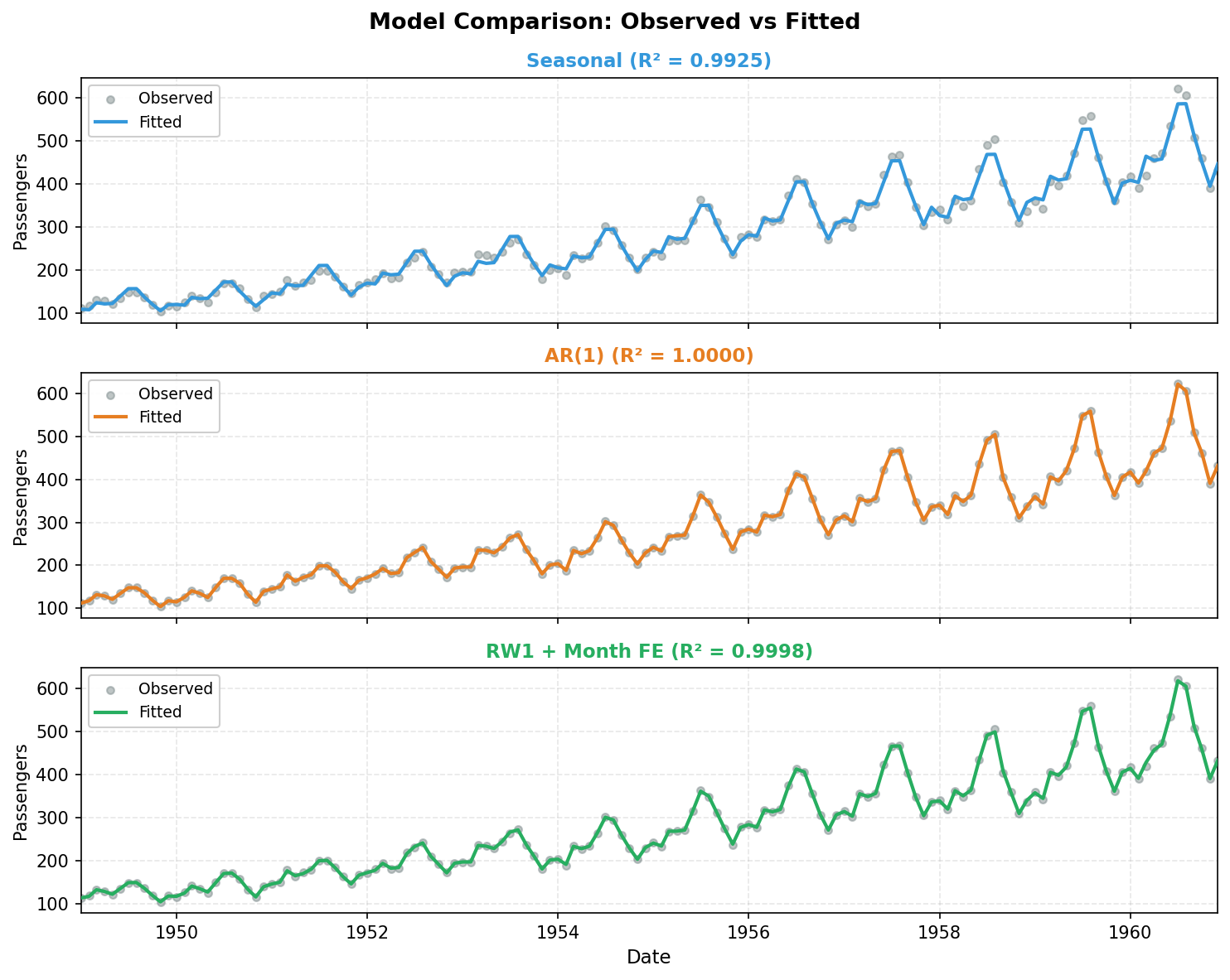
Middle: AR(1): year fixed effects + AR(1) random effect.
Bottom: RW1: month fixed effects + RW1 random effect.
All three models achieve high in-sample fit, but differ in marginal likelihood: RW1 (169.0) > Seasonal (126.7) > AR(1) (42.4). Higher marginal likelihood indicates stronger model evidence under the specified priors and likelihood, balancing fit and complexity.
Key Takeaways
- Seasonal random effects in INLA provide a principled way to model periodic patterns with proper uncertainty quantification.
- Log transformation converts multiplicative seasonality to additive, simplifying the modeling.
- The
season.lengthparameter defines the period (12 for monthly data with yearly cycles). - Year-specific intercepts capture the long-term trend when combined with seasonal effects.
- Multiple model formulations (seasonal, AR1, RW1) can capture different aspects of temporal dependence.
- Model comparison via marginal likelihood helps select the most appropriate model for the data.
References
- Box, G.E.P., Jenkins, G.M., and Reinsel, G.C. (1976). Time Series Analysis: Forecasting and Control. Holden-Day, San Francisco.
- Gomez-Rubio, V. (2020). Bayesian Inference with INLA. Chapman & Hall/CRC Press, Boca Raton, FL.
- Rue, H., Martino, S. and Chopin, N. (2009). "Approximate Bayesian inference for latent Gaussian models using integrated nested Laplace approximations." Journal of the Royal Statistical Society: Series B, 71(2), 319-392.