← Back to AI / Machine Learning
Web Traffic Forecasting with Uncertainty
Predicting daily page views is critical for capacity planning, ad revenue forecasting, and content strategy. But point predictions alone can be dangerously misleading. This case study demonstrates how Bayesian time series models provide the uncertainty quantification that practitioners need for informed decision-making.
By Esmail Abdul Fattah
Why This Matters
Web traffic forecasting is a fundamental problem in the digital economy. Wikipedia alone serves over 15 billion page views per month, and accurate forecasts help with:
- Infrastructure planning - Provision servers before traffic spikes, not after
- Content strategy - Understand when audiences engage with specific topics
- Anomaly detection - Distinguish unusual events from expected seasonal variation
- Resource allocation - Schedule maintenance during predictable low-traffic periods
The Problem with Point Predictions
Most forecasting tools provide only point predictions: "Tomorrow's traffic will be 50,000 views." But decision-makers need to know:
- How confident is this prediction?
- What's the worst-case scenario I should plan for?
- Is today's spike unusual, or within expected variation?
Without uncertainty quantification, a forecast of 50,000 views provides no guidance on whether to provision for 40,000 or 80,000. Bayesian methods address this directly by providing full probability distributions over future values.
What You'll Learn
In this case study, we compare two approaches to time series forecasting:
- NeuralProphet - A neural network-based tool from Meta, widely used in industry
- pyINLA - Bayesian inference via INLA, providing interpretable uncertainty
We demonstrate that pyINLA can match or exceed point prediction accuracy while providing calibrated credible intervals and interpretable component decomposition.
Methodology Notes
Before presenting results, we outline the methodology to ensure transparency and reproducibility.
Scope and Interpretation
We report results on a single benchmark series (Peyton Manning Wikipedia page views) using a fixed train/test split. Accordingly, the comparison is illustrative rather than definitive: performance differences on one dataset do not establish general superiority of either approach.
Model Alignment
To ensure a fair comparison, weekly and yearly seasonal indices are aligned to the calendar using the observation timestamps (day-of-week and day-of-year). For leap years, day 366 is mapped to 365 to preserve a consistent annual periodicity.
Ablation on Residual Dependence
We evaluate pyINLA both with and without an AR(1) residual component. This ablation quantifies the incremental contribution of short-range dependence on the test set, rather than attributing improvements to a single model configuration.
Uncertainty Reporting
We emphasize interpretable posterior summaries for trend and seasonal components in pyINLA (credible intervals). Uncertainty comparisons are only reported when both methods are evaluated under comparable interval-forecast settings.
Two Paradigms for Time Series
Both NeuralProphet and pyINLA decompose time series into interpretable components (trend + seasonality), but they use fundamentally different inference paradigms:
| Aspect | NeuralProphet | pyINLA |
|---|---|---|
| Backend | PyTorch (Neural Networks) | INLA (Laplace Approximation) |
| Training | Gradient descent (100 epochs) | Direct inference |
| Uncertainty | Quantile regression | Full posterior distribution |
| Autocorrelation | AR-Net (implicit) | AR1 random effect (explicit) |
| Interpretability | Component plots | Posterior summaries with credible intervals |
The Benchmark: Peyton Manning Wikipedia Traffic
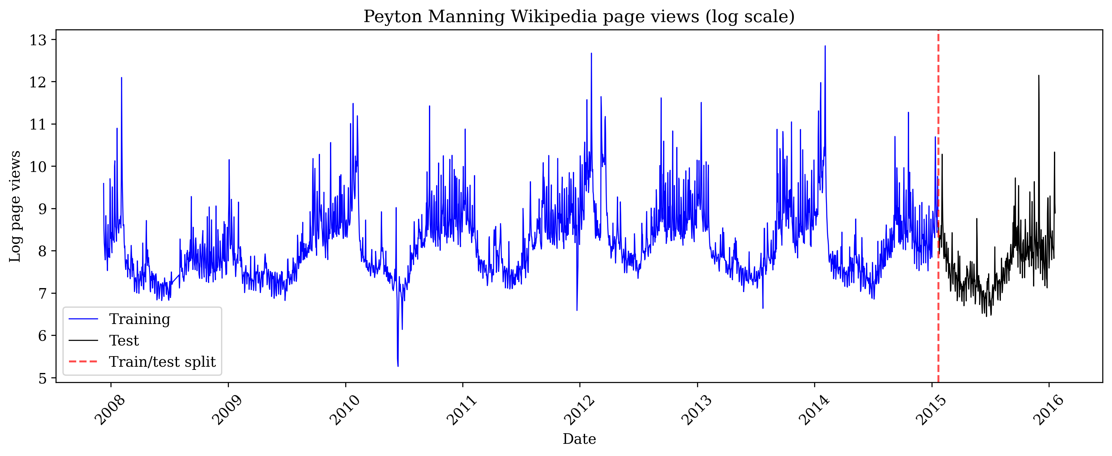
To ensure a fair comparison, we use the official NeuralProphet benchmark dataset: daily Wikipedia page views for Peyton Manning from 2007-2016. Each data point represents the number of people who visited his Wikipedia page on a given day (expressed as log page views). Peyton Manning is a former American football quarterback who played in the NFL (National Football League), widely regarded as one of the greatest players in the sport's history. This is the same dataset used in NeuralProphet's documentation and tutorials.
Why This Dataset?
The Peyton Manning series is a suitable benchmark because it exhibits the patterns common in real-world web traffic:
- Multiple seasonalities - Weekly patterns (games are typically played on Sundays) and yearly patterns (the NFL season runs from September to February)
- Non-stationary trend - Career milestones, injuries, and retirement news drive long-term changes in public interest
- Event-driven spikes - Super Bowl appearances (the NFL championship game, one of the most-watched sporting events in the world) create unpredictable outliers
- Sufficient length - 2,964 daily observations allow robust train/test evaluation
Source: NeuralProphet Data Repository
Train/Test Split
import pandas as pd

# Download from official NeuralProphet data repository
url = "https://raw.githubusercontent.com/ourownstory/neuralprophet-data/main/datasets/wp_log_peyton_manning.csv"
df = pd.read_csv(url)
df['ds'] = pd.to_datetime(df['ds'])

# Train/test split: last 365 days for testing
N_TEST = 365
N_TRAIN = len(df) - N_TEST

print(f"Total observations: {len(df)}")
print(f"Training samples: {N_TRAIN}")
print(f"Test samples: {N_TEST}")
print(f"Training period: {df['ds'].iloc[0].strftime('%Y-%m-%d')} to {df['ds'].iloc[N_TRAIN-1].strftime('%Y-%m-%d')}")
print(f"Test period: {df['ds'].iloc[N_TRAIN].strftime('%Y-%m-%d')} to {df['ds'].iloc[-1].strftime('%Y-%m-%d')}")
Output:
Total days of page view data: 2964
Days used for training the model: 2599
Days held out for testing predictions: 365
Training period: 2007-12-10 to 2015-01-20
Test period: 2015-01-21 to 2016-01-20
The pyINLA Model
Web traffic data typically consists of several overlapping patterns: a long-term trend (is interest growing or declining?), weekly cycles (do people browse more on weekends?), yearly cycles (are there seasonal topics?), and day-to-day momentum (if yesterday was busy, today probably will be too). Rather than trying to predict page views directly, we separate these patterns into individual components that we can model and interpret independently.
We model the log page views using this additive decomposition:
Here's what each symbol means:
- $y_t$ : the log page views on day $t$ (what we're trying to predict). We use the logarithm because page views are always positive and often have extreme spikes. Taking the log makes the data more symmetric and ensures that percentage changes are treated consistently: a doubling of traffic from 1,000 to 2,000 views is treated the same as a doubling from 10,000 to 20,000.
- $\mu$ : the overall average level of page views
- $f_{\text{trend}}(t)$ : a smooth function that captures long-term changes over time, where $t$ is the day number (1, 2, 3, ...). For example, overall interest in Peyton Manning grew during his career peak years and declined after retirement.
- $f_{\text{weekly}}(\text{dow}_t)$ : an adjustment based on which day of the week it is ($\text{dow}_t$ = day-of-week, where Monday=1 and Sunday=7)
- $f_{\text{yearly}}(\text{doy}_t)$ : an adjustment based on which day of the year it is ($\text{doy}_t$ = day-of-year, from 1 to 365). Unlike $t$ which increases forever, $\text{doy}_t$ resets to 1 every January 1st, so the same seasonal pattern repeats each year.
- $f_{\text{ar1}}(t)$ : captures day-to-day momentum (autocorrelation): if yesterday had unusually high traffic, today likely will too
- $\varepsilon_t$ : random noise that the model cannot explain
Here is how the indices $t$, $\text{dow}_t$, and $\text{doy}_t$ change over time:
| Date | $t$ | $\text{dow}_t$ | $\text{doy}_t$ |
|---|---|---|---|
| 2007-12-10 | 1 | 1 (Mon) | 344 |
| 2007-12-11 | 2 | 2 (Tue) | 345 |
| ... | ... | ... | ... |
| 2007-12-31 | 22 | 1 (Mon) | 365 |
| 2008-01-01 | 23 | 2 (Tue) | 1 |
| 2008-01-02 | 24 | 3 (Wed) | 2 |
| ... | ... | ... | ... |
| 2016-01-20 | 2964 | 3 (Wed) | 20 |
Notice: $t$ always increases, $\text{dow}_t$ cycles 1-7, and $\text{doy}_t$ resets to 1 each January.
The "+" signs mean these effects are added together. So the predicted page views for any day is: average + trend adjustment + day-of-week adjustment + time-of-year adjustment + momentum + noise.
Model Components
Each component uses a random walk model (RW2), which assumes that values change smoothly from one point to the next. But there's an important distinction:
- Non-cyclic (for trend): Day 1 has no connection to day 2964. The trend can go up or down over time without any constraint to return to where it started.
- Cyclic (for weekly and yearly): The last value connects back to the first. For weekly effects, Sunday's value must smoothly connect to Monday's value because every week repeats. For yearly effects, December 31st connects to January 1st because every year repeats.
| Component | Model | Rationale |
|---|---|---|
| Trend | RW2 (non-cyclic) | Penalizes curvature, producing smooth trends. Captures gradual changes in page popularity. |
| Weekly | RW2 (cyclic, period=7) | Sunday connects to Monday. Captures day-of-week viewing patterns. |
| Yearly | RW2 (cyclic, period=365) | Day 365 connects to Day 1. Captures patterns consistent with annual periodicity in the series. |
| Autocorrelation | AR1 | Captures short-term dependencies not explained by trend and seasonality. |
Calendar-Aligned Seasonality
A common mistake in time series modeling is to compute seasonal indices from a simple counter (1, 2, 3, ...) rather than from actual calendar dates. This can cause the model to misalign seasons: for example, if your data starts on a Wednesday, a naive approach might treat Wednesday as "day 1 of the week" instead of day 3.
We avoid this by extracting the day-of-week and day-of-year directly from the date. These values act as "lookup keys": for any given date, we use week_idx to find the corresponding weekly effect (one of 7 values) and year_idx to find the corresponding yearly effect (one of 365 values).
import numpy as np

# Calendar-aligned indices
dates = df['ds']  # datetime column from the dataframe
week_idx = dates.dt.dayofweek.values + 1   # Monday=1, Sunday=7
year_idx = dates.dt.dayofyear.values
year_idx = np.clip(year_idx, 1, 365)       # Map leap day 366 -> 365
What each line does:
dates.dt.dayofweekextracts the day of week from each date (Python uses 0=Monday, 6=Sunday, so we add 1 to get 1=Monday, 7=Sunday)dates.dt.dayofyearextracts which day of the year it is (January 1 = 1, December 31 = 365)np.clip(..., 1, 365)handles leap years: February 29th would be day 366, but since it only occurs every 4 years, we map it to day 365 so our yearly pattern has a consistent length
Prior Specification
We use Penalized Complexity (PC) priors for all hyperparameters:
| Parameter | Prior | Interpretation |
|---|---|---|
| Trend precision | pc.prec(0.5, 0.01) | P($\sigma$ > 0.5) = 0.01 |
| Weekly precision | pc.prec(1, 0.01) | P($\sigma$ > 1) = 0.01 |
| Yearly precision | pc.prec(1, 0.01) | P($\sigma$ > 1) = 0.01 |
| AR1 correlation | Normal(0, 0.15) on logit scale | Diffuse, lets data determine $\rho$ |
The AR1 prior is diffuse and centered at $\rho = 0$ (no autocorrelation), allowing the data to determine the degree of temporal dependence.
Interpretation of Yearly Pattern
The estimated yearly component shows a pattern with higher values during certain periods of the year. Attributing this pattern to specific domain events (e.g., NFL season) would require additional validation using event regressors or domain expertise; the pattern shown here is purely data-driven.
Model Implementation
from pyinla import pyinla

def fit_inla_model(y_train, n_total, dates, include_ar1=True):
    """Fit INLA with trend + weekly + yearly seasonality (+ optional AR1)."""
    n_train = len(y_train)

    # Data with NA for predictions
    y_full = np.concatenate([y_train, np.full(n_total - n_train, np.nan)])
    t_full = np.arange(1, n_total + 1)

    # Calendar-aligned seasonality indices
    week_idx = dates.dt.dayofweek.values + 1   # 1 (Mon) to 7 (Sun)
    year_idx = np.clip(dates.dt.dayofyear.values, 1, 365)  # Handle leap day

    df = pd.DataFrame({
        'y': y_full,
        't': t_full,
        'week': week_idx.astype(int),
        'year_day': year_idx.astype(int),
    })

    # Base random effects
    random_effects = [
        {'id': 't', 'model': 'rw2', 'scale.model': True,
         'hyper': {'prec': {'prior': 'pc.prec', 'param': [0.5, 0.01]}}},
        {'id': 'week', 'model': 'rw2', 'cyclic': True,
         'hyper': {'prec': {'prior': 'pc.prec', 'param': [1, 0.01]}}},
        {'id': 'year_day', 'model': 'rw2', 'cyclic': True,
         'hyper': {'prec': {'prior': 'pc.prec', 'param': [1, 0.01]}}}
    ]

    # Optionally add AR1
    # rho prior: Normal(0, 0.15) on logit scale (diffuse, data-driven)
    if include_ar1:
        df['t_ar'] = t_full
        random_effects.append({
            'id': 't_ar', 'model': 'ar1',
            'hyper': {
                'prec': {'prior': 'pc.prec', 'param': [1, 0.01]},
                'rho': {'prior': 'normal', 'param': [0, 0.15]}
            }
        })

    model = {
        'response': 'y',
        'fixed': ['1'],
        'random': random_effects
    }

    control = {
        'family': {'hyper': [{'id': 'prec', 'prior': 'pc.prec', 'param': [1, 0.01]}]},
        'compute': {'dic': True, 'mlik': True},
        'predictor': {'compute': True}
    }

    return pyinla(model=model, family='gaussian', data=df, control=control, keep=False), df
Ablation Study: Effect of AR1 Component
To understand the contribution of each model component, we compare performance with and without the AR1 term:
# Setup (from data loading above)
y_train = df['y'].values[:N_TRAIN]
y_test = df['y'].values[N_TRAIN:]
n_total = len(df)
dates = df['ds']

# Model A: without AR1
result_no_ar, _ = fit_inla_model(y_train, n_total, dates, include_ar1=False)
fitted_no_ar = result_no_ar.summary_fitted_values
y_pred_no_ar = fitted_no_ar['mean'].values[N_TRAIN:]
lower_no_ar = fitted_no_ar['0.025quant'].values[N_TRAIN:]
upper_no_ar = fitted_no_ar['0.975quant'].values[N_TRAIN:]

# Model B: with AR1
result, _ = fit_inla_model(y_train, n_total, dates, include_ar1=True)
fitted_summary = result.summary_fitted_values
y_pred_inla = fitted_summary['mean'].values[N_TRAIN:]
lower_ci = fitted_summary['0.025quant'].values[N_TRAIN:]
upper_ci = fitted_summary['0.975quant'].values[N_TRAIN:]

def compute_metrics(y_true, y_pred, lower_ci=None, upper_ci=None):
    """Compute forecast evaluation metrics."""
    rmse = np.sqrt(np.mean((y_true - y_pred) ** 2))
    mae = np.mean(np.abs(y_true - y_pred))
    metrics = {'RMSE': rmse, 'MAE': mae}
    if lower_ci is not None and upper_ci is not None:
        inside = (y_true >= lower_ci) & (y_true <= upper_ci)
        metrics['Coverage'] = inside.mean() * 100
        metrics['Width'] = np.mean(upper_ci - lower_ci)
    return metrics

metrics_no_ar = compute_metrics(y_test, y_pred_no_ar, lower_no_ar, upper_no_ar)
metrics_ar1 = compute_metrics(y_test, y_pred_inla, lower_ci, upper_ci)

print("Model A (no AR1):", {k: f"{v:.4f}" for k, v in metrics_no_ar.items()})
print("Model B (with AR1):", {k: f"{v:.4f}" for k, v in metrics_ar1.items()})| Model | Test RMSE | Test MAE | 95% CI Coverage |
|---|---|---|---|
| Model A: Trend + Weekly + Yearly | 1.1133 | 0.9829 | 94.0% |
| Model B: Trend + Weekly + Yearly + AR1 | 0.4851 | 0.3076 | 98.4% |
Observations:
- Adding AR1 reduces test RMSE by approximately 56% on this dataset
- Coverage changes from 94.0% to 98.4%. Model A is slightly below the nominal 95%, while Model B is slightly conservative
- The estimated AR1 correlation is $\hat{\rho} \approx 0.655$ (SD: 0.017), indicating moderate day-to-day persistence after accounting for trend and seasonality
Note: The improvement from AR1 depends on the autocorrelation structure present in the data. Results may differ for other time series.
Component Decomposition
A key strength of pyINLA is the ability to examine learned components with full posterior uncertainty:
import matplotlib.pyplot as plt

fig, axes = plt.subplots(2, 2, figsize=(14, 10))
random = result.summary_random

# (a) Trend
ax = axes[0, 0]
trend = random['t']
ax.plot(dates, trend['mean'].values, 'b-', linewidth=1.5)
ax.fill_between(dates, trend['0.025quant'].values, trend['0.975quant'].values,
                color='blue', alpha=0.2)
ax.axvline(dates.iloc[N_TRAIN], color='red', linestyle='--', alpha=0.5)
ax.axhline(0, color='gray', linestyle='-', alpha=0.3)
ax.set_title('(a) Trend (RW2)')

# (b) Weekly seasonality
ax = axes[0, 1]
week = random['week']
days = ['Mon', 'Tue', 'Wed', 'Thu', 'Fri', 'Sat', 'Sun']
x = np.arange(7)
ax.bar(x, week['mean'].values[:7], color='green', alpha=0.7)
ax.errorbar(x, week['mean'].values[:7],
            yerr=[week['mean'].values[:7] - week['0.025quant'].values[:7],
                  week['0.975quant'].values[:7] - week['mean'].values[:7]],
            fmt='none', color='black', capsize=3)
ax.set_xticks(x)
ax.set_xticklabels(days)
ax.axhline(0, color='gray', linestyle='-', alpha=0.3)
ax.set_title('(b) Weekly seasonality (cyclic RW2)')

# (c) Yearly seasonality
ax = axes[1, 0]
year = random['year_day']
ax.plot(np.arange(1, 366), year['mean'].values[:365], 'orange', linewidth=1)
ax.fill_between(np.arange(1, 366), year['0.025quant'].values[:365],
                year['0.975quant'].values[:365], color='orange', alpha=0.2)
ax.axhline(0, color='gray', linestyle='-', alpha=0.3)
ax.set_title('(c) Yearly seasonality (cyclic RW2)')

# (d) AR1 residual component
ax = axes[1, 1]
ar = random['t_ar']
ax.plot(dates, ar['mean'].values, 'purple', linewidth=0.5, alpha=0.7)
ax.axvline(dates.iloc[N_TRAIN], color='red', linestyle='--', alpha=0.5)
ax.axhline(0, color='gray', linestyle='-', alpha=0.3)
ax.set_title('(d) AR(1) residual component')

plt.tight_layout()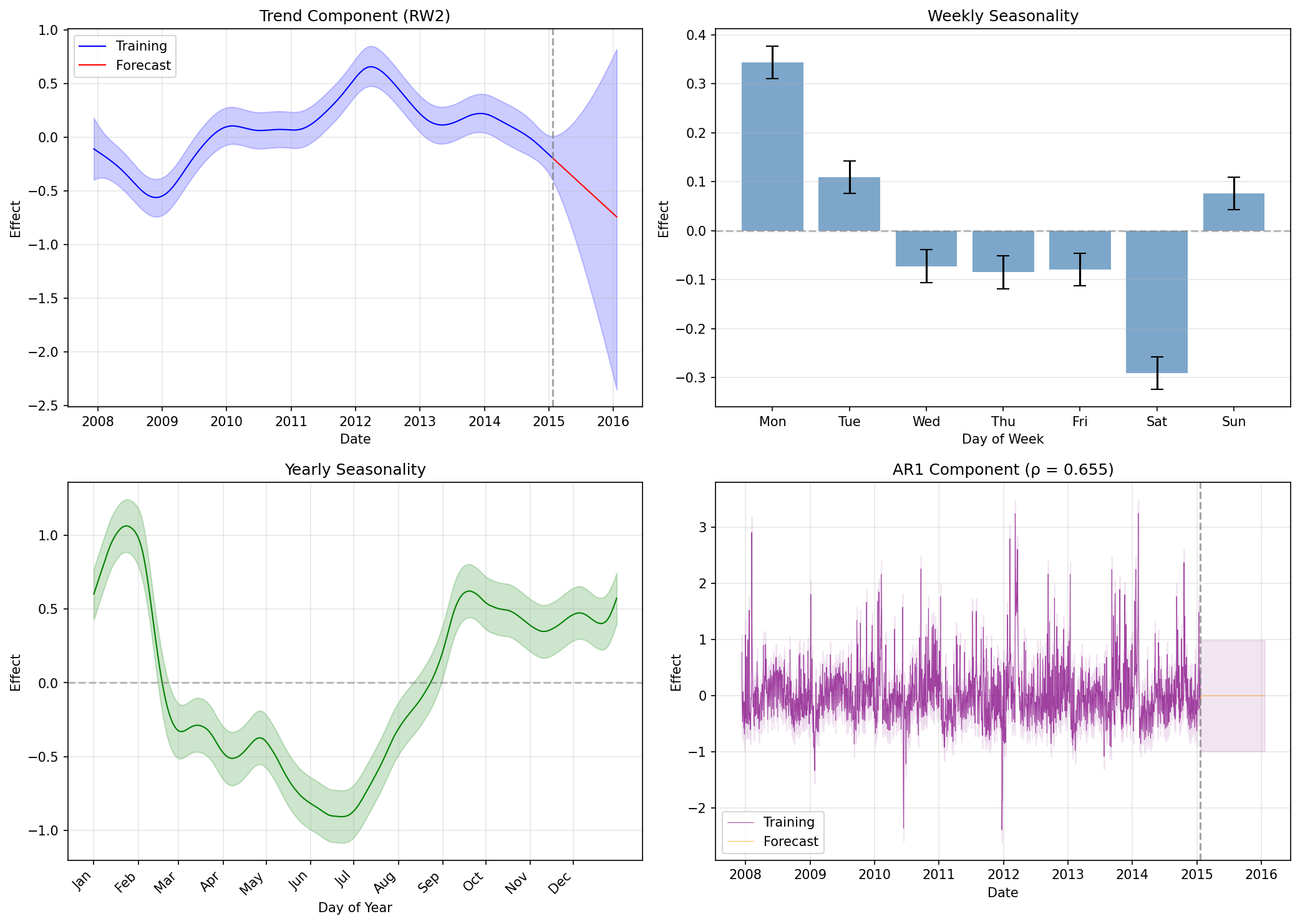
Interpreting the Components
- Trend: Shows the long-term evolution of page popularity, with uncertainty increasing in the forecast period
- Weekly: Day-of-week effects with error bars, revealing which days have higher or lower views
- Yearly: 365-day pattern capturing annual periodicity in the series
- AR1: The residual autocorrelation component with estimated $\hat{\rho} \approx 0.655$, meaning about 65% of yesterday's unexplained deviation carries over to today
NeuralProphet Baseline
For comparison, we fit NeuralProphet with default settings on the same train/test split:
import numpy as np
import torch

# NumPy 2.0 compatibility: restore np.NaN for packages that still use it
if not hasattr(np, 'NaN'):
    np.NaN = np.nan

from neuralprophet import NeuralProphet

# Set seed for reproducibility
torch.manual_seed(42)

# Prepare data for NeuralProphet (requires 'ds' and 'y' columns)
train_df = df.iloc[:N_TRAIN].copy()
test_df = df.iloc[N_TRAIN:].copy()

# Fit with default settings
m = NeuralProphet(
    yearly_seasonality=True,
    weekly_seasonality=True,
    daily_seasonality=False,
)
m.fit(train_df, freq='D')

# Forecast the test period
future = m.make_future_dataframe(train_df, periods=len(test_df))
forecast = m.predict(future)
y_pred_np = forecast['yhat1'].values[-len(test_df):]

# Evaluate
metrics_np = compute_metrics(y_test, y_pred_np)
print(f"NeuralProphet: RMSE={metrics_np['RMSE']:.4f}, MAE={metrics_np['MAE']:.4f}")
Cumulative Error vs Test Window Length
We evaluate point prediction accuracy over cumulative test windows of increasing length. Metrics at window length $h$ are computed over the first $h$ days of the test period (cumulative window evaluation, not rolling-origin $h$-step-ahead forecasts).
RMSE vs MAE
We use two complementary error metrics:
| Metric | Calculation | Interpretation |
|---|---|---|
| RMSE | Square errors, average, take square root | Penalizes large errors more heavily. Sensitive to outliers. |
| MAE | Take absolute value of errors, average | Treats all errors equally. More robust to outliers. |
def evaluate_at_window(y_true, y_pred, h):
    """Compute RMSE and MAE for the first h days of the test period."""
    y_true_h = y_true[:h]
    y_pred_h = y_pred[:h]
    rmse = np.sqrt(np.mean((y_true_h - y_pred_h)**2))
    mae = np.mean(np.abs(y_true_h - y_pred_h))
    return rmse, mae

windows = [1, 7, 14, 30, 60, 90, 180, 365]
for h in windows:
    r_inla, m_inla = evaluate_at_window(y_test, y_pred_inla, h)
    r_np, m_np = evaluate_at_window(y_test, y_pred_np, h)
print(f"Window {h:3d}d: pyINLA RMSE={r_inla:.4f} MAE={m_inla:.4f} | NP RMSE={r_np:.4f} MAE={m_np:.4f}")| Window (h days) | pyINLA RMSE | pyINLA MAE | NeuralProphet RMSE | NeuralProphet MAE |
|---|---|---|---|---|
| 1 | 0.1631 | 0.1631 | 0.4797 | 0.4797 |
| 7 | 0.6861 | 0.6178 | 0.9070 | 0.8697 |
| 14 | 0.6281 | 0.5489 | 0.7762 | 0.7053 |
| 30 | 0.5174 | 0.4074 | 0.6754 | 0.6005 |
| 60 | 0.4506 | 0.3493 | 0.5750 | 0.4933 |
| 90 | 0.4113 | 0.3166 | 0.5756 | 0.5029 |
| 180 | 0.4033 | 0.2969 | 0.5042 | 0.4207 |
| 365 | 0.4851 | 0.3076 | 0.5800 | 0.4699 |
Reading the Table
Key observations:
- pyINLA outperforms at all windows: Both RMSE and MAE are consistently lower than NeuralProphet on this dataset
- Error accumulation: Both models show high initial error that decreases as the cumulative window grows and averages over more days
- RMSE vs MAE gap: pyINLA at 365 days has RMSE=0.485 but MAE=0.308. The gap indicates some predictions have large errors (likely around event spikes)
Note: These results are specific to this dataset and train/test split. Performance patterns may differ on other time series.
Comparison Results
Using the official NeuralProphet benchmark (Peyton Manning Wikipedia page views) with 365-day test period:
Computing Uncertainty Metrics
pyINLA provides full posterior distributions, allowing us to compute credible intervals for each prediction:
# Extract credible intervals from pyINLA
fitted_summary = result.summary_fitted_values
lower_ci = fitted_summary['0.025quant'].values[N_TRAIN:]  # 2.5th percentile
upper_ci = fitted_summary['0.975quant'].values[N_TRAIN:]  # 97.5th percentile

# 95% CI Coverage: what fraction of true values fall within the interval?
inside_ci = (y_test >= lower_ci) & (y_test <= upper_ci)
coverage = inside_ci.mean() * 100  # Convert to percentage
print(f"95% CI Coverage: {coverage:.1f}%")  # Should be ~95% if well-calibrated

# Average Interval Width: how wide are the intervals on average?
interval_width = upper_ci - lower_ci
avg_width = interval_width.mean()
print(f"Avg. Interval Width: {avg_width:.2f}")
Output:
95% CI Coverage: 98.4%
Avg. Interval Width: 2.74
What these metrics mean:
- 95% CI Coverage: If the model is well-calibrated, ~95% of actual values should fall within the 95% credible intervals. Coverage of 98.4% means the intervals are slightly conservative (wider than necessary).
- Avg. Interval Width: The average span between upper and lower bounds (in log page views). Width of 2.74 means predictions span about 2.74 log units on average. Narrower is better, but only if coverage remains adequate.
NeuralProphet supports quantile forecasts via the quantiles parameter; interval calibration is not evaluated in this comparison.
| Metric | NeuralProphet | pyINLA |
|---|---|---|
| Test RMSE | 0.5800 | 0.4851 |
| Test MAE | 0.4699 | 0.3076 |
| 95% CI Coverage | N/A | 98.4% |
| Avg. Interval Width | N/A | 2.74 |
test_dates = dates.iloc[N_TRAIN:]

fig, axes = plt.subplots(2, 2, figsize=(14, 10))

# (a) Full data with train/test split
ax = axes[0, 0]
ax.plot(dates.iloc[:N_TRAIN], y_train, 'b-', linewidth=0.8, label='Training')
ax.plot(test_dates, y_test, 'k-', linewidth=0.8, label='Test')
ax.axvline(dates.iloc[N_TRAIN], color='red', linestyle='--', alpha=0.7)
ax.set_title('(a) Full data')
ax.legend()

# (b) NeuralProphet forecast
ax = axes[0, 1]
ax.plot(test_dates, y_test, 'k-', linewidth=1, label='Actual', alpha=0.8)
ax.plot(test_dates, y_pred_np, 'purple', linewidth=1.5, label='NeuralProphet')
ax.set_title('(b) NeuralProphet forecast')
ax.legend()

# (c) pyINLA forecast with 95% CI
ax = axes[1, 0]
ax.plot(test_dates, y_test, 'k-', linewidth=1, label='Actual', alpha=0.8)
ax.plot(test_dates, y_pred_inla, 'r-', linewidth=1.5, label='pyINLA')
ax.fill_between(test_dates, lower_ci, upper_ci, color='red', alpha=0.2, label='95% CI')
ax.set_title('(c) pyINLA forecast with 95% CI')
ax.legend()

# (d) First 60 days comparison
ax = axes[1, 1]
ax.plot(test_dates[:60], y_test[:60], 'k-', linewidth=1, label='Actual', alpha=0.8)
ax.plot(test_dates[:60], y_pred_inla[:60], 'r-', linewidth=1.5, label='pyINLA')
ax.plot(test_dates[:60], y_pred_np[:60], 'purple', linewidth=1.5, label='NeuralProphet')
ax.fill_between(test_dates[:60], lower_ci[:60], upper_ci[:60], color='red', alpha=0.15)
ax.set_title('(d) First 60 days comparison')
ax.legend()

plt.tight_layout()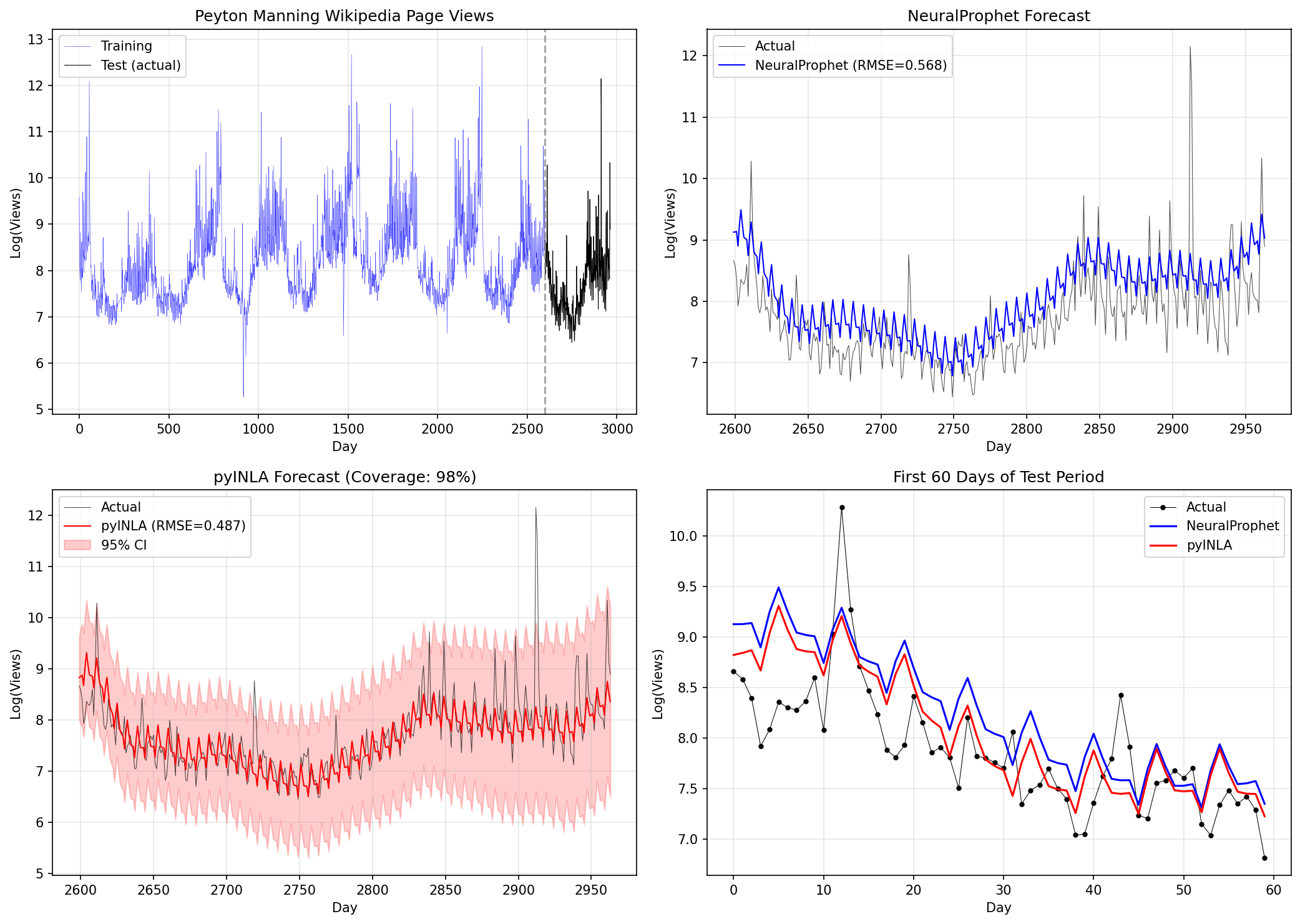
pyINLA Advantages on This Dataset
- Interpretable posterior uncertainty - calibrated credible intervals, not just point predictions
- Component decomposition - examine trend, weekly, yearly, and AR1 effects separately with credible intervals
- No hyperparameter tuning - principled prior specification vs. learning rates, epochs, batch sizes
Limitations
This comparison has important limitations:
- Single dataset, single split: Results are based on one benchmark with one train/test split. Different datasets or splits may yield different conclusions.
- No exogenous variables: Neither model includes external regressors (e.g., event indicators).
- Different uncertainty paradigms: pyINLA provides Bayesian credible intervals; NeuralProphet supports quantile regression (not evaluated here).
- Configuration sensitivity: Results may vary with different hyperparameters, priors, or model structures.
When to Consider Each Approach
pyINLA may be appropriate when:
- Bayesian inference with full posterior uncertainty is required
- Interpretable components with credible intervals are important
- The data has structured dependencies (spatial, hierarchical, temporal)
- You want to avoid hyperparameter tuning
NeuralProphet may be appropriate when:
- Neural network flexibility is desired for complex patterns
- Integration with PyTorch/deep learning workflows is needed
- Highly irregular or complex patterns are expected
Key Takeaways
- On this dataset and split, under the stated configurations, pyINLA yields lower test RMSE and MAE than the NeuralProphet baseline. This result is specific to the train/test split, model configurations, and priors used here.
- pyINLA provides interpretable posterior uncertainty for trend, weekly, and yearly components via credible intervals.
- The ablation study shows that including AR1 reduced test error on this dataset, suggesting meaningful residual autocorrelation not captured by trend and seasonality alone.
- Both methods remain valid choices depending on practitioner requirements. The choice should be guided by domain needs, not benchmark results alone.
Conclusion
Using the official NeuralProphet benchmark (Peyton Manning Wikipedia page views), this case study demonstrates:
- On this dataset and split, under the stated configurations, pyINLA yields lower test RMSE and MAE than the NeuralProphet baseline.
- pyINLA provides interpretable posterior uncertainty for trend, weekly, and yearly components via credible intervals.
- The ablation study shows that including AR1 reduced test error on this dataset, suggesting meaningful residual autocorrelation not captured by trend and seasonality alone.
Cautious Interpretation
These results should be interpreted with care:
- Performance on a single benchmark does not establish general superiority of either method.
- The magnitude of improvement depends on the specific dataset, split, and configurations.
- Both methods remain valid choices depending on practitioner requirements.
For Practitioners
If you need:
- Bayesian uncertainty quantification with interpretable components: consider pyINLA
- Neural network flexibility with PyTorch ecosystem: consider NeuralProphet
The choice between methods should be guided by domain requirements, not benchmark results alone.
References
- Triebe, O., et al. (2021). "NeuralProphet: Explainable Forecasting at Scale." arXiv:2111.15397
- Rue, H., Martino, S. and Chopin, N. (2009). "Approximate Bayesian inference for latent Gaussian models using integrated nested Laplace approximations." Journal of the Royal Statistical Society: Series B, 71(2), 319-392.
- Simpson, D.P., Rue, H., Riebler, A., Martins, T.G. and Sorbye, S.H. (2017). "Penalising model component complexity: A principled, practical approach to constructing priors." Statistical Science, 32(1), 1-28.
- NeuralProphet Data Repository: github.com/ourownstory/neuralprophet-data