Gamma Distribution

Parametrization

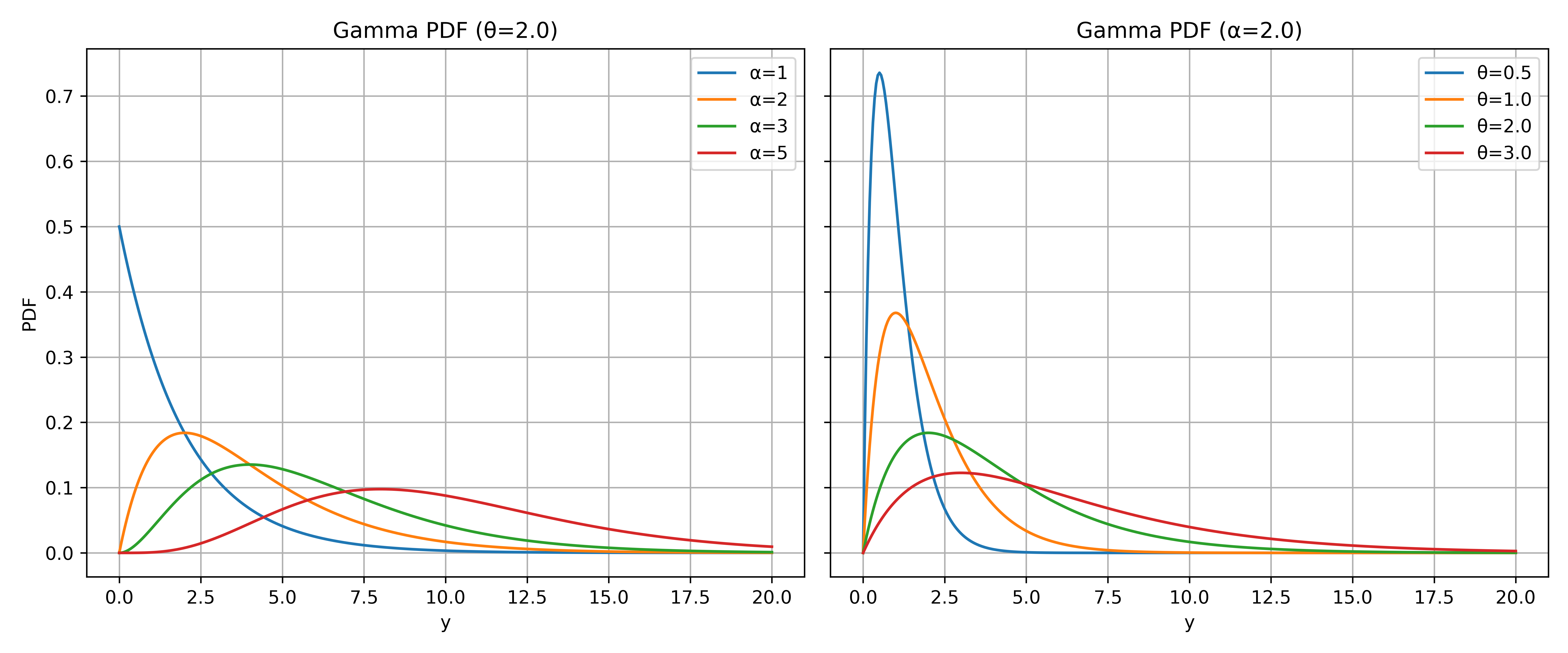
The probability density function (PDF) for the Gamma distribution, considering \(\pmb{y} = (y_1, y_2, \ldots, y_n)\) as a vector of positive continuous responses, is given by:

\[f(y_i \mid a_i, b_i) = \frac{b_i^{a_i}}{\Gamma(a_i)} \, y_i^{a_i-1} \exp(-b_i y_i), \quad y_i > 0, \; a_i > 0, \; b_i > 0, \; i = 1, 2, \ldots, n,\]

where:

• \(\pmb{y} = (y_1, y_2, \ldots, y_n)\) represents the observed positive responses.
• \(\pmb{a} = (a_1, a_2, \ldots, a_n)\) represents the shape parameters.
• \(\pmb{b} = (b_1, b_2, \ldots, b_n)\) represents the rate parameters.

In the regression model, these parameters are linked to the mean vector \(\pmb{\mu} = (\mu_1, \mu_2, \ldots, \mu_n)\), precision parameter \(\phi\), and scale vector \(\pmb{s} = (s_1, s_2, \ldots, s_n)\) through:

\[a_i = s_i \phi, \qquad b_i = \frac{s_i \phi}{\mu_i}, \quad i = 1, 2, \ldots, n,\]

where \(\phi > 0\) is the precision parameter (or \(1/\phi\) is the dispersion parameter) and \(s_i \geq 0\) is a fixed per-observation scaling factor (see the Scale Vector validation rule below). Substituting these relationships yields the density:

\[f(y_i \mid \mu_i, \phi, s_i) = \frac{1}{\Gamma(s_i\phi)} \left(\frac{s_i\phi}{\mu_i}\right)^{s_i\phi} y_i^{s_i\phi - 1} \exp\left(-s_i\phi \frac{y_i}{\mu_i}\right), \quad i = 1, 2, \ldots, n.\]

Mean and Variance

The mean and variance of the Gamma distribution are:

\[\text{E}(y_i) = \mu_i = \frac{a_i}{b_i}, \qquad \text{Var}(y_i) = \frac{a_i}{b_i^2} = \frac{\mu_i^2}{s_i \phi}, \quad i = 1, 2, \ldots, n.\]

The variance is proportional to the square of the mean, a characteristic property of the Gamma distribution. The scale vector \(\pmb{s}\) allows for heterogeneous dispersion across observations, enabling observation-specific variance adjustments while sharing a common precision parameter \(\phi\).

Link Function

The mean vector \(\pmb{\mu}\) is linked to the linear predictor \(\pmb{\eta} = (\eta_1, \eta_2, \ldots, \eta_n)\) using the log link function:

\[\mu_i = \exp(\eta_i), \quad i = 1, 2, \ldots, n,\]

or in vector form:

\[\pmb{\mu} = \exp(\pmb{\eta}).\]

Available link functions depend on the model variant:

• Regression (gamma): default, log, quantile
• Survival (gammasurv): default, log, neglog, quantile

The neglog link, available in survival models, corresponds to the accelerated failure time (AFT) parameterization: \(\lambda_i = \exp(-\eta_i)\), where positive coefficients increase expected survival times.

Hyperparameters

The Gamma likelihood has a single hyperparameter controlling the precision. The precision parameter \(\phi\) is represented on the log scale:

\[\theta = \log(\phi), \qquad \phi = \exp(\theta),\]

and the prior is defined on \(\theta\).

Hyperparameter \(\theta\) (precision)

The default configuration assigns a log-gamma prior to \(\theta\) with shape and rate parameters \((1, 0.01)\). For family="gamma" the initial value is set to \(\theta = \log(100) \approx 4.605\), corresponding to \(\phi = 100\). For family="gammasurv" the initial value is \(\theta = \log(1) = 0\), corresponding to \(\phi = 1\). The prior is relatively diffuse, allowing the precision to adapt during model fitting.

Key: prec (positional aliases: theta, theta1)

When translated into control['family']['hyper'], the default entry is:

control = {
    'family': {
        'hyper': [
            {
                'prior': 'loggamma',
                'param': [1.0, 0.01],
                'initial': 4.605,
                'fixed': False,
            }
        ]
    }
}

Survival Model

The Gamma survival model (gammasurv) extends the regression model to handle time-to-event data with censoring. Survival analysis addresses the challenge of incomplete observation: subjects may exit the study before experiencing the event of interest, resulting in censored observations where only partial information about survival times is available.

Censoring Types

• Right censoring: The event has not occurred by the end of observation; the subject survived at least until the censoring time.
• Left censoring: The event occurred before observation began.
• Interval censoring: The event occurred within a known time interval.

Model Characteristics

The Gamma distribution's shape parameter enables flexible hazard functions:

• Increasing hazard (shape > 1): Risk increases over time, suitable for aging or wear-out processes.
• Constant hazard (shape = 1): Reduces to the exponential distribution.
• Decreasing hazard (shape < 1): Risk decreases over time, appropriate for infant mortality or burn-in failures.

Cure Models

The survival variant exposes 10 additional stratum-slope hyperparameters \(\beta_1, \ldots, \beta_{10}\) for cure-model specifications. Cure models account for a population fraction that will never experience the event of interest. Each \(\beta_i\) has a \(\text{Normal}(-4, 100)\) prior on \(\beta_1\) and \(\text{Normal}(0, 100)\) on \(\beta_2, \ldots, \beta_{10}\); all are estimated by default (fixed=False). Initial values are \(\beta_1 = -7\), \(\beta_2 = \ldots = \beta_{10} = 0\). Most survival users leave these defaults in place and only configure prec.

Survival Response

When using gammasurv, the response must be created using inla_surv():

from pyinla import inla_surv

# Create survival response (event=1 observed, event=0 right-censored)
y_surv = inla_surv(time=df["time"], event=df["event"])
result = pyinla(model={'response': y_surv, 'fixed': ['1', 'x']},
                family="gammasurv", data=df)

Specification

• family="gamma" for regression models
• family="gammasurv" for survival models
• Required arguments:
  • For gamma: \(\pmb{y}\) (response vector) and optionally \(\pmb{s}\) (scale vector, default = 1)
  • For gammasurv: \(\pmb{y}\) provided via inla_surv()

The scale vector \(\pmb{s}\) is not used for gammasurv.

Validation Rules

pyINLA enforces several validation rules for Gamma models to ensure correct specification:

Response Values

Response variable \(\pmb{y}\) must be strictly positive (> 0). Zero or negative values are not allowed.

Hyperparameter Configuration

Key: control['family']['hyper']

When providing hyperparameter configuration for the precision parameter:

• The block must be a list of dicts (the dict-of-named form is not accepted).

• Allowed keys per entry: id, prior, param, initial, fixed. Any other key raises a SafetyError.

• If id is given, it must be one of prec, theta, or theta1.

• Omitted fields fall back to the schema defaults; we recommend setting prior explicitly when you override param or initial.

# Valid hyperparameter configuration
control = {
    'family': {
        'hyper': [{
            'prior': 'loggamma',
            'param': [1.0, 0.01],
            'initial': 4.605,
            'fixed': False
        }]
    }
}

Allowed Priors

Key: control['family']['hyper'][i]['prior']

For family="gamma", the precision hyperparameter accepts:

• loggamma (default) - Log-gamma prior on log-precision. Requires two positive parameters (shape, rate).

• pc.prec - Penalized complexity prior for precision. Requires two parameters \((u, \alpha)\) with \(P(\sigma > u) = \alpha\).

• User-defined forms with prefix expression:, table:, or rprior: pass through unchecked.

Any other prior name raises a SafetyError.

# Using PC prior for precision
control = {
    'family': {
        'hyper': [{
            'prior': 'pc.prec',
            'param': [1.0, 0.01]  # P(sigma > 1) = 0.01
        }]
    }
}

Scale Vector

Key: scale

When providing the scale argument:

• All values must be non-negative (NaN is rejected). pyINLA mirrors R-INLA here; both accept zero entries.

• Length must match the number of observations.

• Only accepted for gamma; passing scale with gammasurv raises a SafetyError.

# With scale vector
result = pyinla(
    data=df,
    model={'response': 'y', 'fixed': ['1', 'x']},
    family='gamma',
    scale=df['weights'].to_numpy(),
)

Link Functions

Key: control['family']['link']

Available link functions depend on the model variant:

• gamma: log (default), quantile

• gammasurv: log (default), neglog, quantile

Quantile Link Requirements

Key: control['family']['link']

When using the quantile link function:

• Must specify model='quantile' in the control.link configuration

• Must provide quantile parameter strictly between 0 and 1 (exclusive)

# Using quantile link for median regression (quantile = 0.5)
control = {
    'family': {
        'control.link': {
            'model': 'quantile',
            'quantile': 0.5,
        }
    }
}
result = pyinla(
    data=df,
    model={'response': 'y', 'fixed': ['1', 'x']},
    family='gamma',
    control=control,
)

• Gamma Regression