Gamma Regression

Introduction

In this tutorial, we fit a Bayesian Gamma regression model for positive continuous data. The Gamma distribution is the natural choice when modeling strictly positive outcomes where the variance increases with the mean, such as insurance claims, waiting times, or rainfall amounts.

The Gamma likelihood uses a log-link function to ensure positive predictions, and includes a precision hyperparameter that controls the dispersion of the data around the mean.

The Model

We consider a Gamma regression model with $n$ observations. For each observation $i = 1, \ldots, n$, the positive response $y_i$ is modeled as:

y_i \sim \text{Gamma}(a_i, b_i)

where the shape $a_i$ and rate $b_i$ parameters are related to the mean $\mu_i$ and precision parameter $\phi$ through:

a_i = s_i \phi, \qquad b_i = \frac{s_i \phi}{\mu_i}

Here:

$y_i > 0$ is the positive continuous response
$\mu_i > 0$ is the mean
$\phi > 0$ is the precision parameter (hyperparameter)
$s_i > 0$ is an optional per-observation scale factor (default = 1)

The density function is:

\pi(y_i) = \frac{1}{\Gamma(s_i\phi)} \left(\frac{s_i\phi}{\mu_i}\right)^{s_i\phi} y_i^{s_i\phi - 1} \exp\left(-s_i\phi \frac{y_i}{\mu_i}\right)

Linear Predictor

The linear predictor $\eta_i$ links to the mean through a log-link function:

\eta_i = \beta_0 + \beta_1 x_i

where $\beta_0$ is the intercept and $\beta_1$ is the slope coefficient for covariate $x_i$.

The Gamma distribution uses the log link function (default), so the mean is:

\mu_i = \exp(\eta_i)

This ensures that the predicted mean is always positive.

Likelihood Function

The likelihood for the full dataset $\mathbf{y} = (y_1, \ldots, y_n)^\top$ is:

p(\mathbf{y} \mid \boldsymbol{\beta}, \phi, \mathbf{s}) = \prod_{i=1}^{n} \frac{1}{\Gamma(s_i\phi)} \left(\frac{s_i\phi}{\mu_i}\right)^{s_i\phi} y_i^{s_i\phi - 1} \exp\left(-s_i\phi \frac{y_i}{\mu_i}\right)

where $\mu_i = \exp(\beta_0 + \beta_1 x_i)$ and $\boldsymbol{\beta} = (\beta_0, \beta_1)^\top$.

Hyperparameters

The Gamma likelihood has one hyperparameter: the precision parameter $\phi$. It is internally represented as:

\phi = \exp(\theta)

where the prior is placed on $\theta$. The default prior is a log-gamma with parameters (1, 0.01).

The variance of the Gamma distribution is:

\text{Var}(y_i) = \frac{\mu_i^2}{s_i \phi}

So larger values of $\phi$ correspond to smaller variance (more precision).

Dataset

The dataset contains $n = 1000$ observations with three columns:

Column	Description	Type
`y`	Positive continuous response	float
`x`	Covariate (predictor variable)	float
`scale`	Per-observation scale factor	float

dataset_gamma_regression.csv

Download the CSV file and place it in your working directory.

Implementation in pyINLA

We fit the model using pyINLA. The key steps are:

Load the data into a pandas DataFrame
Extract the scale vector (if using per-observation scaling)
Define the model structure (response and fixed effects)
Call pyinla() with family='gamma' and the scale vector

import pandas as pd
from pyinla import pyinla

# Load data
df = pd.read_csv('dataset_gamma_regression.csv')
scale = df['scale'].to_numpy()

# Define model: y ~ 1 + x (intercept + slope)
model = {
    'response': 'y',
    'fixed': ['1', 'x']
}

# Fit the Gamma regression model
result = pyinla(
    model=model,
    family='gamma',
    data=df,
    scale=scale
)

# View posterior summaries for fixed effects
print(result.summary_fixed)

# View posterior summary for precision parameter
print(result.summary_hyperpar)

Extracting Results

The result object contains all posterior inference:

# Fixed effects: posterior summaries for beta_0 and beta_1
print(result.summary_fixed)

# Extract posterior means
intercept = result.summary_fixed.loc['(Intercept)', 'mean']
slope = result.summary_fixed.loc['x', 'mean']

# Compute predicted means
import numpy as np
eta_hat = intercept + slope * df['x'].to_numpy()
mu_hat = np.exp(eta_hat)

# Hyperparameter: precision parameter phi
print(result.summary_hyperpar)

The summary_fixed DataFrame includes columns for mean, sd, 0.025quant, 0.5quant, 0.975quant, and mode.

Data Generation (Reference)

For reproducibility, the dataset was simulated from the following data-generating process:

x_i \stackrel{\text{iid}}{\sim} \mathcal{N}(0, 1), \quad s_i \sim \text{Uniform}(0.5, 2), \quad y_i \sim \text{Gamma}(a_i, b_i)

where $\eta_i = \beta_0 + \beta_1 x_i$, $\mu_i = \exp(\eta_i)$, $a_i = s_i \phi$, and $b_i = \mu_i / a_i$.

True parameter values: $\beta_0 = 1$, $\beta_1 = 1$, $\phi = 1.2$.

# Data generation script (for reference only)
import numpy as np
import pandas as pd

rng = np.random.default_rng(2026)
n = 1000
beta0, beta1 = 1.0, 1.0
phi = 1.2  # precision parameter

x = rng.normal(size=n)
eta = beta0 + beta1 * x
mu = np.exp(eta)
scale = rng.uniform(0.5, 2, size=n)

# Gamma parameters
a = phi * scale  # shape
b = mu / a       # scale (not rate!)
y = rng.gamma(shape=a, scale=b)

df = pd.DataFrame({'y': y, 'x': np.round(x, 6), 'scale': np.round(scale, 6)})
# df.to_csv('dataset_gamma_regression.csv', index=False)

Results and Diagnostics

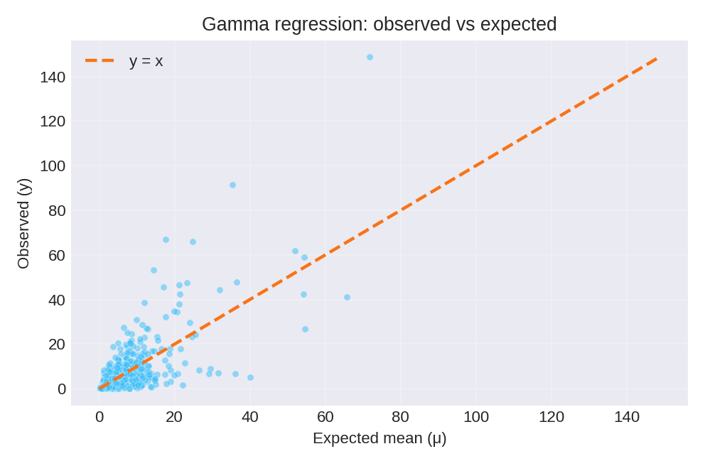
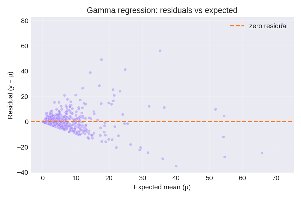
The posterior summaries recover the true parameters: $\beta_0 = 1.0$, $\beta_1 = 1.0$, and precision $\phi = 1.2$. The diagnostic plots below compare observed values with expected means and show the residual pattern.

Observed values versus expected means with identity line — Observed values $y_i$ versus expected means $\hat{\mu}_i = \exp(\hat{\eta}_i)$.

Residuals versus expected means — Residuals $y_i - \hat{\mu}_i$ versus expected means.

To reproduce these figures locally, download the render_gamma_plots.py script and run it alongside the CSV dataset.