Gaussian Distribution

Parametrization

The probability density function (PDF) for the Gaussian distribution is expressed as:

\[\label{eq:gaussian-pdf} f(\pmb{y}) = \left( \frac{\sqrt{s\tau}}{\sqrt{2\pi}} \right)^n \, \exp\!\Bigl( -\tfrac{1}{2} \, s\tau \, (\pmb{y} - \pmb{\mu})^T (\pmb{y} - \pmb{\mu}) \Bigr),\]

where:

• \(\pmb{y} \in \mathbb{R}^n\) is a vector of observed values.

• \(\pmb{\mu} \in \mathbb{R}^n\) is the vector of means corresponding to each element of \(\pmb{y}\).

• \(s\) is a positive scaling factor that modifies the overall precision of the distribution.

• For \(s = 1\), \(\tau\) is the precision, defined as the inverse of the variance \(\tau = 1/\sigma^2\).

• \(n\) is the number of observations (the dimension of \(\pmb{y}\)).

To illustrate how different parameter settings (mean \(\mu\), variance \(\sigma^2\), precision \(\tau\), and scale \(s\)) influence the shape of the Gaussian distribution, Figure 1 displays several overlaid Gaussian curves.

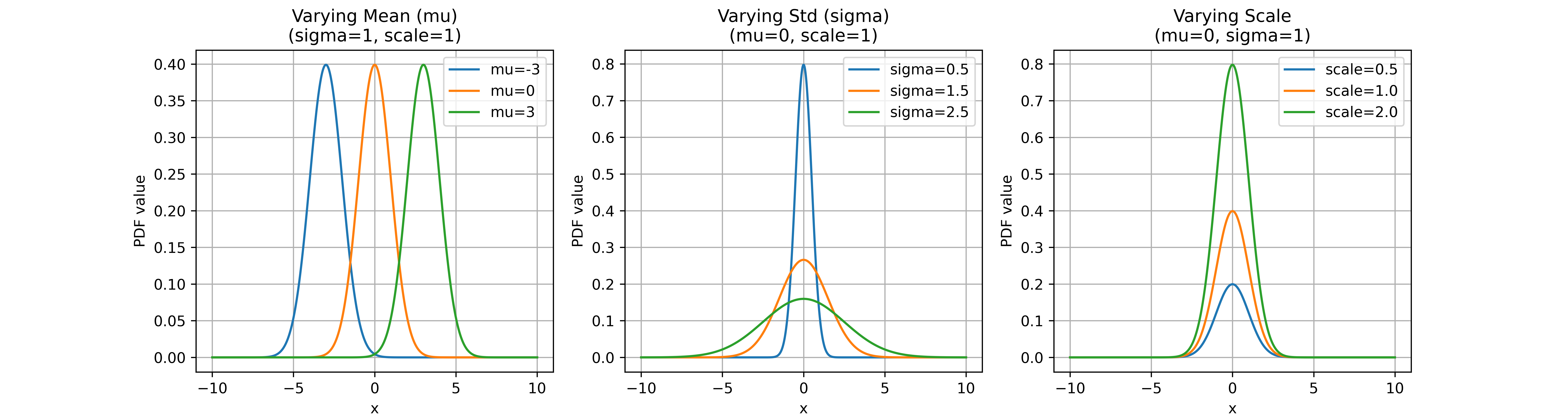
As seen in the figure, increasing \(\sigma^2\) (i.e., decreasing \(\tau\)) broadens the Gaussian curve, while decreasing \(\sigma^2\) makes it narrower and taller. Likewise, shifting \(\mu\) moves the location of the peak along the x-axis. The additional scale factor \(s\) can also expand or contract the distribution as needed for certain modeling contexts.

Mean and Variance

The mean vector \(\pmb{\mu}\) is directly linked to the linear predictor \(\pmb{\eta}\) via an identity link function:

\[\pmb{\mu} = \pmb{\eta}.\]

The variance of the distribution, \(\sigma^2\), is defined as:

\[\sigma^2 = \frac{1}{s \tau},\]

where \(\tau\) is the precision, controlling the spread or dispersion of the distribution. In the simplest case (isotropic covariance), the covariance matrix is \(\sigma^2 I_n\).

Link Function

The mean of the response is linked to the linear predictor \(\pmb{\eta} = (\eta_1, \eta_2, \dots, \eta_n)\) through a link function. The default is the identity link:

\[\mu_i = \eta_i.\]

Possible link functions: identity (default), logit, log, cauchit, loga.

To specify a non-default link, use control={'family': {'link': 'log'}}. The loga link additionally requires the a parameter via control['family']['control.link'] = {'a': <value in (0, 1]>}. Omit link entirely to use the default identity link.

Hyperparameters

In a Bayesian framework for Gaussian likelihood models, hyperparameters typically control the precision \(\tau\) (inverse of the variance) or other variance-related quantities. These hyperparameters often appear as log-transformed parameters to ensure they remain within valid (positive) ranges and to improve numerical stability during inference.

Within pyINLA, the Gaussian likelihood collects these in the hyperparameter vector \(\boldsymbol{\theta} = (\theta_1, \theta_2)\). The first entry, \(\theta_1\), controls the main precision term and is always present. The second entry, \(\theta_2\), is optional and contributes an offset precision component; when not needed, it is omitted or fixed so that its effect on \(\tau\) is negligible.

Hyperparameter \(\theta_1\) (precision)

Key: prec

By default, the model uses: \[\tau = \kappa_1,\] where \(\kappa_1\) is a positive parameter that we often represent via the log-transformation: \[\theta_1 = \log(\kappa_1).\] Thus, \(\theta_1\) can take on any real value, ensuring \(\kappa_1>0\). In practice, \(\theta_1\) is often assigned a prior distribution (e.g., a log-Gamma) to capture prior beliefs about the likely range of \(\tau\). In the default configuration (captured in the dictionary below), this hyperparameter is labelled “log precision”, starts at 4, is estimated rather than fixed, and sets prior="loggamma" with param=[1, 5e-5], which corresponds to a log-gamma prior with those shape and rate values. These defaults imply that, initially, \(\kappa_1 = e^{\,4}\approx 54.6\), with a broad log-Gamma prior that allows the precision \(\tau\) to adapt during model fitting.

Hyperparameter \(\theta_2\) (precision offset)

Key: precoffset (fixed by default)

Some models introduce a second hyperparameter \(\kappa_2\) to incorporate additional variance or offset terms in the precision. Its log-transformed version is: \[\theta_2 = \log(\kappa_2).\] This leads to a precision defined by \[\frac{1}{\tau} = \frac{1}{\kappa_1} + \frac{1}{\kappa_2},\] which equivalently becomes \[\tau = \frac{1}{(1/\kappa_1) + (1/\kappa_2)}.\] Hence, \(\tau\) depends on both \(\kappa_1\) and \(\kappa_2\). For instance, if \(1/\kappa_2\) is negligible (i.e., effectively zero), we recover \(\tau \approx \kappa_1\). When this hyperparameter is used, the default configuration (see dictionary below) labels it “log precision offset”, assigns the large initial value 72.087, fixes it during optimisation, and leaves prior and parameters unset, reflecting that it is only there to guard against numerical issues.

In many implementations, a practical threshold classifies \(1/\kappa_2\) as zero if it falls below machine epsilon. Numerically, this is equivalent to \(\theta_2 \geq 36.04\) (since \(\log(1/\varepsilon_{\mathrm{mach}}) \approx 36.044\)), beyond which the contribution of \(\kappa_2\) to \(\tau\) is effectively nil. For this reason precoffset must always remain fixed: explicitly setting fixed=False for it raises a safety error.

The offset component is treated as a safety valve: the default keeps it fixed with prior and parameters left unset. Attempting to supply a non-None prior, supply param, or set fixed=False for precoffset raises a safety error.

When translated into control['family']['hyper'], the default entries look like this:

control = {
    'family': {
        'hyper': [
            {
                'id': 'prec',
                'prior': 'loggamma',
                'param': [1.0, 5e-5],
                'initial': 4.0,
                'fixed': False,
            },
            {
                'id': 'precoffset',
                'initial': 72.087,
                'fixed': True,
            },
        ]
    }
}

In summary, by tuning or estimating \(\theta_1\) and \(\theta_2\), one can flexibly control the precision \(\tau\) in a Gaussian likelihood model, allowing for richer or more constrained variance structures based on the application’s requirements.

Validation Rules

pyINLA enforces several validation rules for Gaussian models to ensure correct specification:

Hyperparameter Configuration

Key: control['family']

For the Gaussian family, control['family'] only accepts the key hyper. Any other key raises a safety error.

Each entry in control['family']['hyper'] may only contain these keys:

• id - Hyperparameter identifier (prec or precoffset)

• prior - Prior distribution name

• param - Prior parameters

• initial - Initial value on log scale

• fixed - Whether to fix the hyperparameter

Allowed Priors for Precision

Key: control['family']['hyper'] entry with 'id': 'prec'

The precision hyperparameter (prec) accepts any prior from the prior registry. The most commonly useful choices for a positive precision are:

The precision can also be pinned at a known value by setting fixed=True (no prior required). Unknown prior names raise a clear pyinla safety check: unknown prior '...' error before the engine runs, with a "Did you mean ..." hint for typos. Wrong param length similarly trips a safety error.

# With loggamma prior (default)
control = {
    'family': {
        'hyper': [{
            'id': 'prec',
            'prior': 'loggamma',
            'param': [1.0, 0.01],
            'initial': 2.0
        }]
    }
}

# With pc.prec prior
control = {
    'family': {
        'hyper': [{
            'id': 'prec',
            'prior': 'pc.prec',
            'param': [1.0, 0.01],
            'initial': 4.0,
            'fixed': False,
        }]
    }
}

# With normal prior on log-precision
control = {
    'family': {
        'hyper': [{
            'id': 'prec',
            'prior': 'normal',
            'param': [0.0, 0.001],   # mean, precision (sd ~= 31.6)
        }]
    }
}

# Improper flat prior (no shrinkage; param must be empty)
control = {
    'family': {
        'hyper': [{
            'id': 'prec',
            'prior': 'flat',
            'param': [],
        }]
    }
}

# Fixed at a known precision value
control = {
    'family': {
        'hyper': [{
            'id': 'prec',
            'initial': 4.0,  # log(prec), so prec = exp(4.0) ~ 55
            'fixed': True
        }]
    }
}

Precision Offset Restrictions

Key: control['family']['hyper'] entry with 'id': 'precoffset'

The precoffset hyperparameter has special restrictions:

• Must remain fixed=True

• Prior must be None, the string "none", or omitted

• Cannot specify custom param

import math

# Fixed known variance component var0
control = {
    'family': {
        'hyper': [{
            'id': 'precoffset',
            'initial': math.log(1.0 / var0),  # log(1/var0)
            'fixed': True
        }]
    }
}

# Combined: estimated prec + fixed precoffset
control = {
    'family': {
        'hyper': [
            {
                'id': 'prec',
                'prior': 'loggamma',
                'param': [1.0, 5e-5],
                'initial': 4.0
            },
            {
                'id': 'precoffset',
                'initial': math.log(1.0 / var0),
                'fixed': True
            }
        ]
    }
}

Scale Vector

Key: scale

When using the scale argument, all values must be strictly positive (> 0).

# With observation-specific scale
model = {'response': 'y', 'fixed': ['1', 'x']}
result = pyinla(model=model, data=df, family="gaussian", scale=df["weights"])

Specification

• family="gaussian"

• Required arguments:

  • \(\pmb y\): observed values (\(y_i \in \mathbb{R}\) for each observation).

• Gaussian Regression: Log-Gamma Prior
• Gaussian Regression: Observation Scale
• Gaussian Regression: Precision Offset