Parametrization
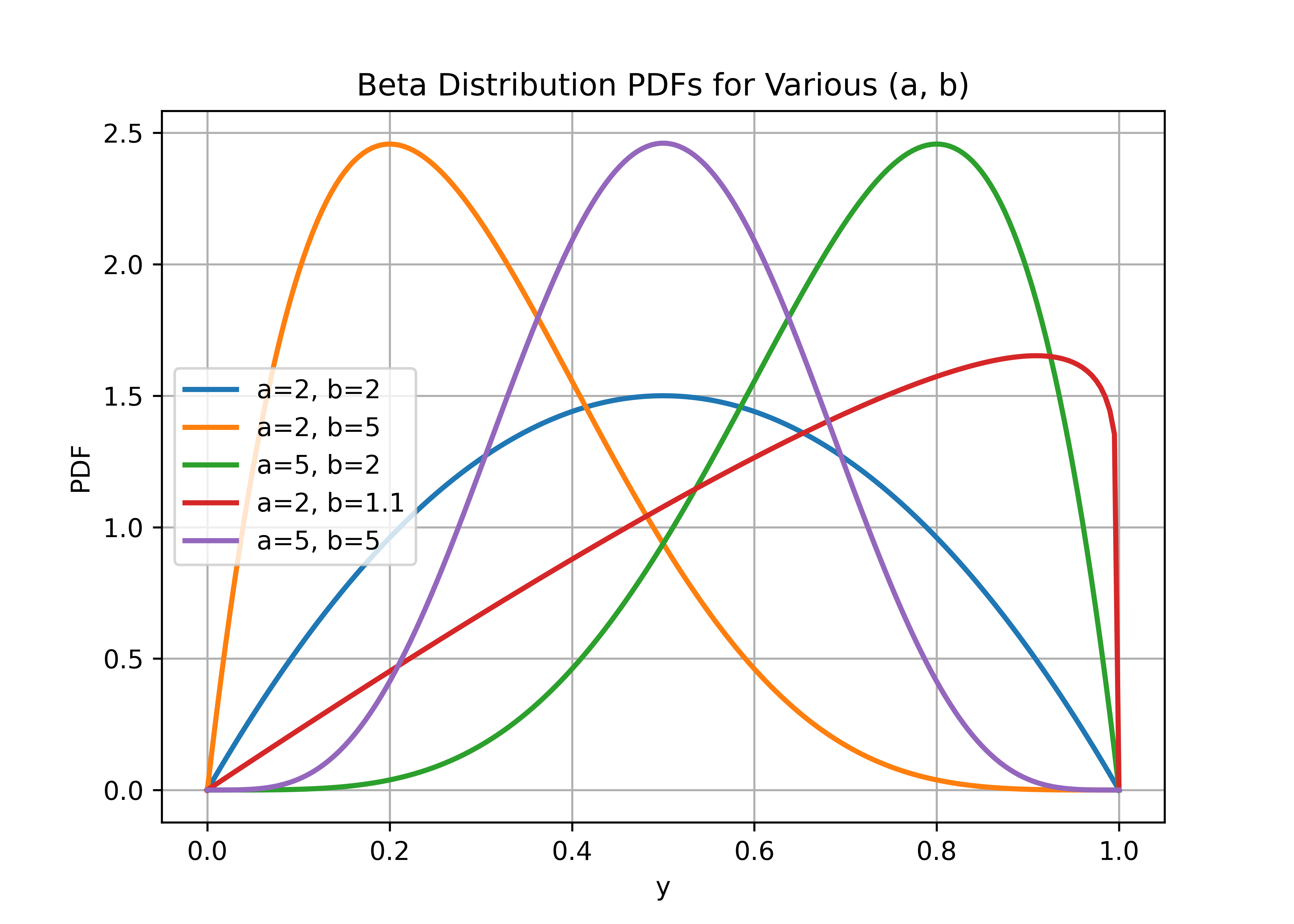
The Beta distribution for a random vector \(\pmb{y} = (y_1, y_2, \dots, y_n)\) of observations on \((0, 1)\) is defined by the probability density function:
\[\pi(y_i) = \frac{1}{B(a_i, b_i)} y_i^{a_i-1}(1-y_i)^{b_i-1}, \quad 0 < y_i < 1, \quad i = 1, 2, \dots, n\]
where \(a_i > 0\) and \(b_i > 0\) are shape parameters, and \(B(a_i, b_i)\) is the Beta function:
\[B(a_i, b_i) = \frac{\Gamma(a_i)\Gamma(b_i)}{\Gamma(a_i+b_i)}\]
Mean and Variance
The Beta distribution is reparameterized using the mean \(\mu_i\) and precision parameter \(\phi_i\):
\[\mu_i = \frac{a_i}{a_i + b_i}, \qquad \phi_i = a_i + b_i, \quad i = 1, 2, \dots, n\]
Under this parameterization, the mean and variance are:
\[\text{E}(y_i) = \mu_i, \qquad \text{Var}(y_i) = \frac{\mu_i(1-\mu_i)}{1+\phi_i}, \quad i = 1, 2, \dots, n\]
The shape parameters are recovered as:
\[a_i = \mu_i \phi_i, \qquad b_i = \phi_i (1-\mu_i), \quad i = 1, 2, \dots, n\]
The precision parameter \(\phi_i\) controls the variance: for fixed \(\mu_i\), larger \(\phi_i\) results in smaller variance.
Link Function
The mean is linked to the linear predictor \(\pmb{\eta} = (\eta_1, \eta_2, \dots, \eta_n)\) using the logit link (default):
\[\mu_i = \frac{\exp(\eta_i)}{1 + \exp(\eta_i)}, \quad i = 1, 2, \dots, n\]
Possible link functions: logit (default), loga, cauchit, probit, cloglog, ccloglog, loglog.
Censoring
In some applications, observations close to 0 or 1 are censored and recorded exactly as 0 or 1. A censoring threshold \(0 < \delta < 0.5\) can be specified:
Observations \(y_i \leq \delta\) are treated as censored at 0.
Observations \(y_i \geq 1 - \delta\) are treated as censored at 1.
By default, no censoring is applied (\(\delta = 0\)).
Hyperparameters
The Beta likelihood has one hyperparameter: the precision parameter \(\phi > 0\). It is represented internally on the log scale:
\[\theta = \log(\phi), \qquad \phi = \exp(\theta)\]
With an optional scale vector \(\pmb{s} = (s_1, s_2, \dots, s_n)\), the observation-specific precision is:
\[\phi_i = s_i \cdot \phi = s_i \exp(\theta), \quad i = 1, 2, \dots, n\]
Hyperparameter \(\theta\) (phi)
The default configuration assigns a loggamma prior to \(\theta\) with shape and rate parameters \((1, 0.1)\). The initial value is set to \(\theta = \log(10) \approx 2.303\).
Key: phi (not prec)
When translated into control['family']['hyper'], the default entry is:
control = {
    'family': {
        'hyper': [{
            'id': 'phi',
            'prior': 'loggamma',
            'param': [1.0, 0.1],
            'initial': 2.303,
            'fixed': False,
        }]
    }
}
Each entry in control['family']['hyper'] may contain these keys:
id- Hyperparameter identifier (phi). Can be omitted for the first (and only) hyperparameter.prior- Prior distribution nameparam- Prior parameters (list)initial- Initial value on log scalefixed- Whether to fix the hyperparameter (True/False)
The precision hyperparameter (phi) accepts any prior from the prior registry. The most commonly useful choices for a positive precision are:
| Prior | Param shape | Use when |
|---|---|---|
loggamma (default) | [shape, rate], both positive | Conjugate prior on the log-precision; widely used. |
pc.prec | [U, alpha] with P(sd > U) = alpha | Penalised-complexity prior on the standard deviation; weakly informative on a meaningful scale. |
normal / gaussian | [mean, precision] on \(\theta\) | Soft Gaussian prior on the log-precision; useful for nudging without strong shrinkage. |
flat | [] | Improper flat. Pass param=[] explicitly. |
logtnormal | [location, scale] | Truncated-normal on \(\theta\); bounded informative prior. |
The precision can also be pinned at a known value by setting fixed=True (no prior required). Unknown prior names raise a clear pyinla safety check: unknown prior '...' error before the engine runs, with a "Did you mean ..." hint for typos. Wrong param length similarly trips a safety error.
Validation Rules
pyINLA enforces several validation rules for beta models to ensure correct specification:
Response Values
Key: response variable
Response values must satisfy:
Without censoring: All values must be strictly in (0, 1) - exclusive bounds
With censoring (
beta.censor.valueset): Values can be in [0, 1] - inclusive bounds
Censoring Threshold (beta.censor.value)
Key: control['family']['beta.censor.value']
When providing the censoring threshold:
Must be in the range [0, 0.5) - values at or above 0.5 are rejected
Default is 0 (no censoring)
# With censoring threshold
model = {"response": "y", "fixed": ["1", "x"]}
result = pyinla(model=model, family="beta", data=df,
                control={"family": {"beta.censor.value": 0.05}})
Scale
Key: scale
When providing the scale argument:
All values must be strictly positive (> 0)
Length must match the number of observations
Hyperparameters
Key: control['family']['hyper']
When configuring hyperparameters:
If
prioris omitted, the schema default is used (loggammawithparam=[1, 0.1]); a fixed entry can also omitpriorandparam.If specified, the prior name must be in the registry (see the table above for the most common choices). Unknown names raise
pyinla safety check: unknown prior.paramlength must match the prior's expected count.
# Custom loggamma prior on precision
model = {"response": "y", "fixed": ["1", "z"]}
control = {
    'family': {
        'hyper': [{
            'id': 'phi',
            'prior': 'loggamma',
            'param': [1.0, 0.5],
            'initial': 1.609,  # log(5), so phi = 5
            'fixed': False
        }]
    }
}
result = pyinla(model=model, family="beta", data=df, scale=scale, control=control)

# PC prior on precision
control = {
    'family': {
        'hyper': [{
            'id': 'phi',
            'prior': 'pc.prec',
            'param': [1.0, 0.01],
            'initial': 1.609,
            'fixed': False
        }]
    }
}
result = pyinla(model=model, family="beta", data=df, scale=scale, control=control)

# Fixed precision (not estimated)
control = {
    'family': {
        'hyper': [{
            'id': 'phi',
            'initial': 2.303,  # log(10), so phi = 10
            'fixed': True
        }]
    }
}
result = pyinla(model=model, family="beta", data=df, scale=scale, control=control)
Exposure Not Allowed
The E (exposure) argument is not allowed for beta. Use nbinomial or poisson if you need exposure.
Ntrials Not Allowed
The Ntrials argument is not allowed for beta. Use binomial or betabinomial if you need trial counts.
Variant Not Allowed
The control['family']['variant'] option is not allowed for beta.
Allowed Link Functions
Key: control['family']['link']
These link functions are supported:
logit(default)logacauchitprobitcloglogccloglogloglog
# With probit link
model = {"response": "y", "fixed": ["1", "x"]}
result = pyinla(model=model, family="beta", data=df,
                control={"family": {"link": "probit"}})
Specification
family="beta"Required arguments: \(\pmb{y}\) (response).
Optional arguments: \(\pmb{s}\) (scale, default = 1) and
beta.censor.value(\(\delta\), default = 0).