Weibull Survival Analysis

Introduction

Survival analysis deals with time-to-event data where some observations may be censored (the event was not observed during the study period). The Weibull distribution is a popular choice for survival models because its hazard function can model increasing, decreasing, or constant hazard rates depending on the shape parameter.

This example demonstrates fitting a Weibull survival model with right-censored data using pyINLA's weibullsurv family and the inla_surv response object.

The Survival Model

For survival data, we observe pairs $(t_i, \delta_i)$ where $t_i$ is the observed time and $\delta_i$ is the event indicator:

• $\delta_i = 1$: Event occurred at time $t_i$
• $\delta_i = 0$: Censored at time $t_i$ (event not yet observed)

The Weibull hazard function is:

The hazard function shape depends on $\alpha$:

• $\alpha < 1$: Decreasing hazard (infant mortality)
• $\alpha = 1$: Constant hazard (exponential distribution)
• $\alpha > 1$: Increasing hazard (aging/wear-out)

Handling Censored Data

The survival likelihood accounts for censoring. For an observation $(t_i, \delta_i)$:

where $f(t)$ is the PDF and $S(t) = 1 - F(t)$ is the survival function.

In pyINLA, this is handled automatically using the inla_surv function to create the survival response object.

Dataset

The dataset contains $n = 1000$ observations with approximately 56% censoring:

• dataset_weibull_surv_v0.csv (Variant 0)
• dataset_weibull_surv_v1.csv (Variant 1)

Implementation in pyINLA

Fitting a Weibull survival model requires using inla_surv to create the survival response:

import pandas as pd
from pyinla import pyinla, inla_surv

# Load survival data
df = pd.read_csv('dataset_weibull_surv_v0.csv')

# Create survival response object
y_surv = inla_surv(
    time=df['y'].to_numpy(),
    event=df['event'].to_numpy()
)

# Define model with survival response
model = {
    'response': y_surv,
    'fixed': ['1', 'x']
}

# Specify variant
control = {
    'family': {
        'variant': 0
    },
    'compute': {
        'dic': True,
        'cpo': True,
        'mlik': True
    }
}

# Fit the survival model
result = pyinla(
    model=model,
    family='weibullsurv',
    data=df,
    control=control
)

# View results
print(result.summary_fixed)
print(result.summary_hyperpar)

Interpreting Results

The fixed effects represent the log-scale relationship with the hazard:

• Intercept ($\beta_0$): Baseline log-scale parameter
• Coefficient ($\beta_1$): Effect of covariate on log($\lambda$)

A positive $\beta_1$ means higher values of $x$ are associated with higher $\lambda$, which corresponds to shorter expected survival times.

The hyperparameter summary shows the posterior for the shape parameter $\alpha$:

• $\alpha \approx 1$: Hazard is approximately constant (exponential model)
• $\alpha > 1$: Hazard increases over time
• $\alpha < 1$: Hazard decreases over time

Using Variant 1

For variant 1 parameterization:

# Load variant 1 data
df_v1 = pd.read_csv('dataset_weibull_surv_v1.csv')

y_surv_v1 = inla_surv(
    time=df_v1['y'].to_numpy(),
    event=df_v1['event'].to_numpy()
)

model_v1 = {'response': y_surv_v1, 'fixed': ['1', 'x']}
control_v1 = {'family': {'variant': 1}}

result_v1 = pyinla(
    model=model_v1,
    family='weibullsurv',
    data=df_v1,
    control=control_v1
)

print(result_v1.summary_fixed)
print(result_v1.summary_hyperpar)

Results and Diagnostics

The posterior summaries provide estimates for $\beta_0$, $\beta_1$, and the shape parameter $\alpha$. The true parameters used for data generation were $\beta_0 = 1.0$, $\beta_1 = 2.2$, and $\alpha = 1.1$.

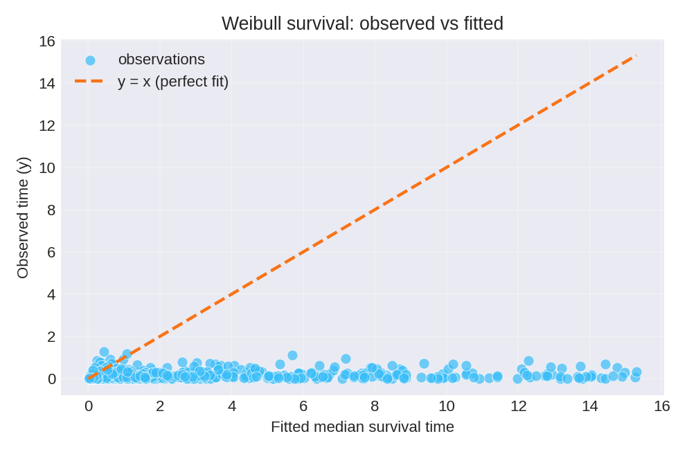
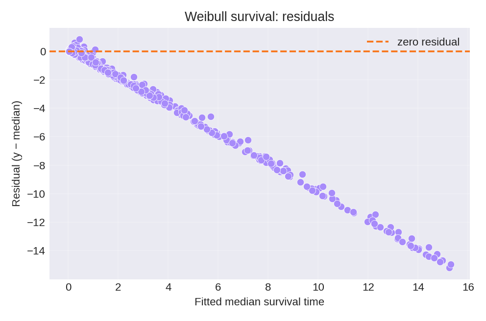
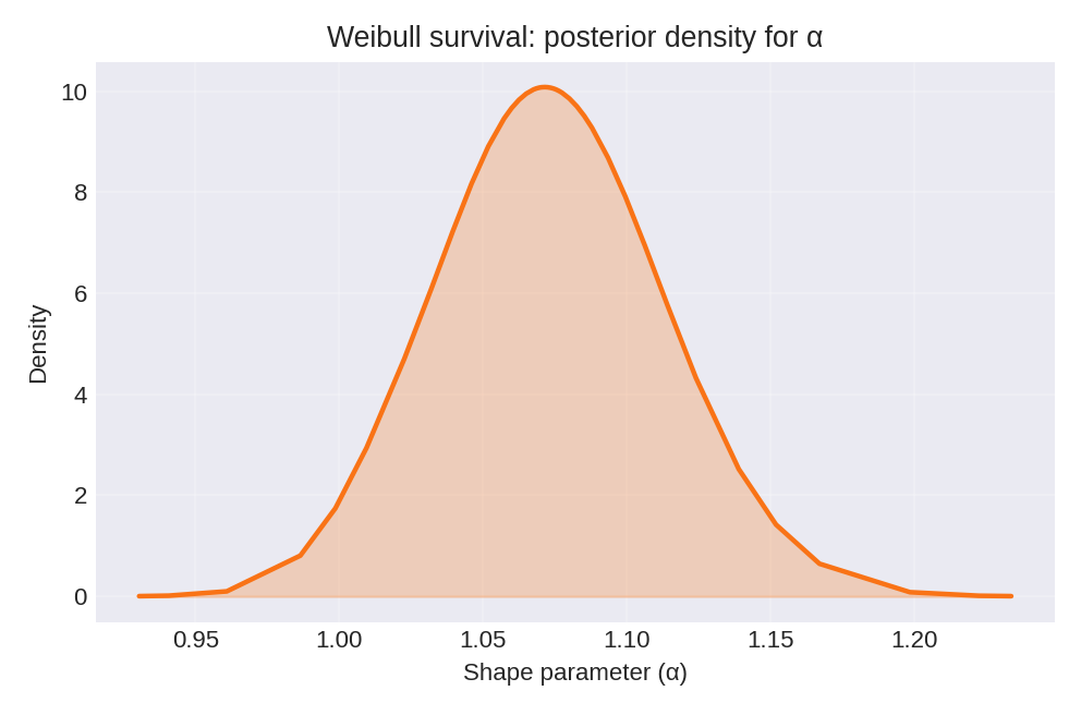
To reproduce these figures locally, download the render_weibullsurv_plots.py script and run it alongside the CSV dataset.

Data Generation (Reference)

The survival data was simulated with random censoring:

# Data generation with censoring
import numpy as np
import pandas as pd

rng = np.random.default_rng(2026)
n = 1000
alpha = 1.1
beta0, beta1 = 1.0, 2.2

x = rng.uniform(-1, 1, size=n)
x = (x - x.mean()) / x.std()

eta = beta0 + beta1 * x
lam = np.exp(eta)

# True event times (variant=0)
scale_v0 = lam ** (-1/alpha)
y_true = rng.weibull(alpha, size=n) * scale_v0

# Censoring times (exponential random censoring)
cens_time = rng.exponential(scale=np.median(y_true), size=n)

# Observed times and event indicator
y_obs = np.minimum(y_true, cens_time)
event = (y_true <= cens_time).astype(int)

df = pd.DataFrame({
    'y': y_obs,
    'x': np.round(x, 6),
    'event': event
})

print(f"Censoring rate: {100 * (1 - event.mean()):.1f}%")
# df.to_csv('dataset_weibull_surv_v0.csv', index=False)

Summary

Key points for Weibull survival analysis in pyINLA:

• Use family='weibullsurv' for survival models with censoring
• Create the response using inla_surv(time, event)
• Choose the appropriate variant (0 or 1) based on your parameterization
• The shape parameter $\alpha$ determines hazard function behavior
• Supports right, left, and interval censoring through the inla_surv object