Weibull Distribution Regression

Introduction

The Weibull distribution is widely used in reliability engineering and survival analysis due to its flexibility in modeling various hazard function shapes. In this example, we fit a Weibull regression model where the response variable represents positive continuous values (e.g., time-to-event data without censoring).

This example demonstrates fitting Weibull regression using both parameterization variants available in pyINLA.

The Model

For each observation $i = 1, \ldots, n$, the response $y_i > 0$ follows a Weibull distribution. Two parameterization variants are available:

Variant 0 (default):

f(y_i) = \alpha y_i^{\alpha - 1} \lambda_i \exp(-\lambda_i y_i^{\alpha})

Variant 1:

f(y_i) = \alpha y_i^{\alpha - 1} \lambda_i^{\alpha} \exp(-(\lambda_i y_i)^{\alpha})

where:

$y_i > 0$ is the positive continuous response
$\alpha > 0$ is the shape parameter (hyperparameter)
$\lambda_i > 0$ is the scale parameter, linked to the linear predictor via $\lambda_i = \exp(\eta_i)$

Linear Predictor

The scale parameter $\lambda_i$ is linked to the covariates through the log link:

\log(\lambda_i) = \eta_i = \beta_0 + \beta_1 x_i

Equivalently:

\lambda_i = \exp(\eta_i) = \exp(\beta_0 + \beta_1 x_i)

Hyperparameters

The shape parameter $\alpha$ is represented internally using a scaled log-transformation:

\alpha = \exp(S \cdot \theta), \quad S = 0.1

The scaling factor $S = 0.1$ improves numerical stability. The default prior is pc.alphaw with parameter 5.

Dataset

The dataset contains $n = 1000$ observations with the following columns:

Column	Description	Type
`y`	Positive continuous response (Weibull distributed)	float
`x`	Covariate (standardized)	float
`event`	Event indicator (all 1s for regression)	int

dataset_weibull_v0.csv (Variant 0)
dataset_weibull_v1.csv (Variant 1)

Implementation in pyINLA

Fitting a Weibull regression model with variant 0:

import pandas as pd
from pyinla import pyinla

# Load data (variant 0)
df = pd.read_csv('dataset_weibull_v0.csv')

# Define model: y ~ 1 + x
model = {
    'response': 'y',
    'fixed': ['1', 'x']
}

# Specify variant in control
control = {
    'family': {
        'variant': 0
    },
    'compute': {
        'dic': True,
        'cpo': True,
        'mlik': True
    }
}

# Fit the model
result = pyinla(
    model=model,
    family='weibull',
    data=df,
    control=control
)

# View results
print(result.summary_fixed)
print(result.summary_hyperpar)

Using Variant 1

For variant 1, simply change the control setting:

# Load data generated with variant 1
df_v1 = pd.read_csv('dataset_weibull_v1.csv')

control_v1 = {
    'family': {
        'variant': 1
    }
}

result_v1 = pyinla(
    model=model,
    family='weibull',
    data=df_v1,
    control=control_v1
)

print(result_v1.summary_fixed)
print(result_v1.summary_hyperpar)

The key difference between variants is how the scale relates to $\lambda$:

Variant 0: scale = $\lambda^{-1/\alpha}$
Variant 1: scale = $1/\lambda$

Results and Diagnostics

The posterior summaries provide estimates for $\beta_0$, $\beta_1$, and the shape parameter $\alpha$. The figures below show the model fit and residual diagnostics for variant 0.

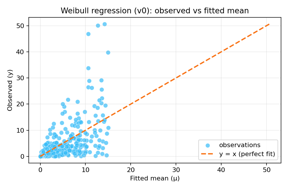
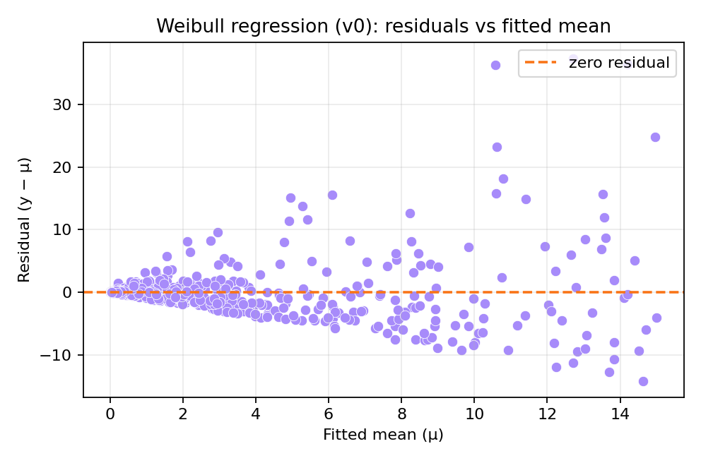
Observed values versus fitted mean with identity line — Observed values $y_i$ versus fitted mean $\hat{\mu}_i$.

Residuals versus fitted mean — Residuals $y_i - \hat{\mu}_i$ versus fitted mean.

To reproduce these figures locally, download the render_weibull_plots.py script and run it alongside the CSV dataset.

Data Generation (Reference)

The dataset was simulated with the following parameters:

\alpha = 1.1, \quad \beta_0 = 1.0, \quad \beta_1 = 2.2

# Data generation (variant 0)
import numpy as np
import pandas as pd

rng = np.random.default_rng(2026)
n = 1000
alpha = 1.1
beta0, beta1 = 1.0, 2.2

# Generate standardized covariate
x = rng.uniform(-1, 1, size=n)
x = (x - x.mean()) / x.std()

# Linear predictor and lambda
eta = beta0 + beta1 * x
lam = np.exp(eta)

# For variant=0: scale = lambda^(-1/alpha)
scale_v0 = lam ** (-1/alpha)
y = rng.weibull(alpha, size=n) * scale_v0

# Create DataFrame
df = pd.DataFrame({
    'y': y,
    'x': np.round(x, 6),
    'event': np.ones(n, dtype=int)
})
# df.to_csv('dataset_weibull_v0.csv', index=False)