Student's t-Distribution: Observation Scale
A tutorial on heteroscedastic robust regression using the Student's t-distribution with observation-specific scale parameters.
Introduction
The Student's t-distribution provides robustness against outliers through its heavier tails. When combined with observation-specific scale parameters, it can also handle heteroscedasticity - situations where different observations have different variances.
This tutorial demonstrates how to fit a t-distribution regression model with observation-specific scale factors in pyINLA, providing both outlier robustness and proper variance modeling.
The Model
For each observation $i = 1, \ldots, n$, the response follows a scaled Student's t-distribution:
where $T_{\nu}$ is a reparameterized Student's t-distribution with unit variance for all values of $\nu > 2$.
The parameters are:
- $y_i \in \mathbb{R}$ is the continuous response variable
- $\eta_i = \beta_0 + \beta_1 x_i$ is the linear predictor (location)
- $\tau > 0$ is the common precision parameter (estimated)
- $s_i > 0$ is the known scale factor for observation $i$ (fixed, not estimated)
- $\nu > 2$ is the degrees of freedom (estimated)
The effective variance for each observation is:
Observations with larger $s_i$ have smaller variance (more precise), while observations with smaller $s_i$ have larger variance (less precise).
When to Use Scale Parameters
Combining the t-distribution with scale parameters is useful when you have:
- Heteroscedastic data with outliers: When variance varies across observations and some extreme values may be present
- Weighted robust regression: When some observations are more reliable than others, but outliers may still occur
- Meta-analysis with heavy tails: When combining studies with different standard errors and potential outlying studies
- Financial data: Asset returns often exhibit both heteroscedasticity and heavy tails
The scale parameter acts as a weight: larger $s_i$ gives more weight to observation $i$, while the t-distribution automatically downweights extreme residuals.
Dataset
The dataset contains $n = 400$ observations with three columns:
| Column | Description | Type |
|---|---|---|
y | Continuous response variable | float |
x | Covariate (predictor variable) | float |
scale | Observation-specific scale factor $s_i$ | float (positive) |
Implementation in pyINLA
To incorporate observation-specific scales with the t-distribution, pass the scale vector to the scale argument:
import pandas as pd
from pyinla import pyinla

# Load data with scale column
df = pd.read_csv('dataset_t_scale.csv')

# Define model: y ~ 1 + x
model = {
    'response': 'y',
    'fixed': ['1', 'x']
}

# Specify control options
control = {
    'compute': {
        'dic': True,
        'cpo': True,
        'mlik': True
    }
}

# Fit the model with observation-specific scales
result = pyinla(
    model=model,
    family='T',  # uppercase T
    data=df,
    scale=df['scale'].to_numpy(),  # Pass scale vector
    control=control
)

# View posterior summaries
print(result.summary_fixed)
print(result.summary_hyperpar)
Important: The scale argument must be a numpy array (or array-like) with the same length as the number of observations. Each element $s_i$ should be positive.
Expected Output
Running the model produces posterior summaries that account for both the heteroscedastic structure and heavy tails:
Fixed Effects
| Parameter | Mean | SD | 2.5% | 97.5% |
|---|---|---|---|---|
| (Intercept) | 0.443 | 0.037 | 0.370 | 0.516 |
| x | 1.467 | 0.037 | 1.395 | 1.539 |
Hyperparameters
| Parameter | Mean | SD | 2.5% | 97.5% |
|---|---|---|---|---|
| Precision for t | 1.133 | 0.134 | 0.892 | 1.418 |
| Degrees of freedom | 4.901 | 1.117 | 3.293 | 7.619 |
The true parameters used for data generation were $\beta_0 = 0.5$, $\beta_1 = 1.5$, $\tau = 1$, and $\nu = 4$. The model successfully recovers these values.
Custom Priors
You can customize priors on the precision and degrees of freedom hyperparameters:
# Custom priors with scale
control = {
    'family': {
        'hyper': [
            {
                'id': 'prec',
                'prior': 'loggamma',
                'param': [1, 0.01],
            },
            {
                'id': 'dof',
                'prior': 'pc.dof',
                'param': [10, 0.5],   # P(nu > 10) = 0.5
            },
        ]
    },
    'compute': {
        'dic': True
    }
}

result = pyinla(
    model=model,
    family='T',
    data=df,
    scale=df['scale'].to_numpy(),
    control=control
)
Data Generation (Reference)
The dataset was simulated with heteroscedastic t-distributed errors:
import numpy as np
import pandas as pd

rng = np.random.default_rng(2028)
n = 400

# Generate covariate
x = rng.normal(0, 1, size=n)

# Linear predictor
eta = 0.5 + 1.5 * x

# Generate heteroscedastic scales
scale = rng.uniform(0.5, 2.0, size=n)

# Degrees of freedom
nu = 4

# Generate t-distributed response with scaling
# With scale s, effective precision is s*tau
# The t is reparameterized for unit variance
t_errors = rng.standard_t(df=nu, size=n)
y = eta + t_errors / (np.sqrt(scale) * np.sqrt(nu / (nu - 2)))

df = pd.DataFrame({
    'y': y,
    'x': np.round(x, 6),
    'scale': np.round(scale, 6)
})
# df.to_csv('dataset_t_scale.csv', index=False)
Interpretation Notes
- Double Robustness: The model provides robustness through both the t-distribution (handling outliers via heavy tails) and the scale parameters (handling heteroscedasticity).
- Reported Precision: The hyperparameter summary reports the base precision $\tau$. The effective precision for observation $i$ is $\tau \cdot s_i$.
- Degrees of Freedom: Lower $\nu$ values indicate heavier tails and more outlier robustness. As $\nu \to \infty$, the t-distribution approaches the Gaussian.
- Unit Variance Reparameterization: The t-distribution in INLA is reparameterized to have unit variance for all $\nu > 2$, simplifying interpretation of the precision parameter.
Results and Diagnostics
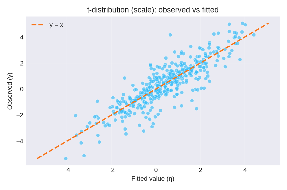
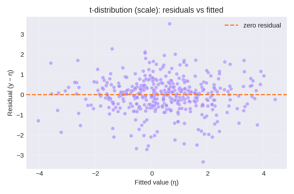
The posterior summaries recover the true parameters: $\beta_0 = 0.5$, $\beta_1 = 1.5$, $\tau = 1$, and $\nu = 4$. The diagnostic plots below compare observed values with fitted values and show the residual pattern.
To reproduce these figures locally, download the render_t_scale_plots.py script and run it alongside the CSV dataset.